PA5 example answers

Setup

Let’s start by loading some libraries.

library("tidyverse")
library("here")
library("broom")
library("knitr")

Now we will load the dataset. It is already downloaded and lives at the root level of my pa5 directory.

dat <- read_csv("ratings_data_2025-04-23.csv")

Rows: 195 Columns: 6
── Column specification ────────────────────────────────────────────────────────
Delimiter: ","
chr  (2): id, comment
dbl  (3): week, enjoy, difficulty
date (1): date

ℹ Use `spec()` to retrieve the full column specification for this data.
ℹ Specify the column types or set `show_col_types = FALSE` to quiet this message.

Ok. Now we are ready to get started. Let’s go straight through the questions.

Questions

I will address each question brielfy. First, I will highlight the main issue the questions presents. Second, I will mention the possible solutions. After, I will go through the process of answering the questions.

Q1 - Enjoyment as a function of class

Problem: The dataset contains repeated measures.
Solution: We will have to use a complicated multilevel model or average over participants/time in order to get a single observation per individual. The latter probably isn’t ideal, but it is a solution the meshes well with what we have done in class, so we will go with that.

# Separate the `date` column to get access to 'year'
# Then group by id and year and calculate the overall average enjoyment for each id
enjoy_avg_id <- dat |>
  separate(date, into = c("year", "month", "day"), sep = "-") |> 
  group_by(id, year) |> 
  summarize(avg_enj = mean(enjoy), .groups = "drop")

# Take a look at the first 6 rows
head(enjoy_avg_id)

# A tibble: 6 × 3
  id            year  avg_enj
  <chr>         <chr>   <dbl>
1 Anon1         2025    0.887
2 Anonymous ID  2023    0.401
3 Anonymous ID  2025    0.702
4 Anonymous ID2 2023    0.458
5 Catling       2023    0.895
6 Dasani        2025    0.544

Now the data is in a useable format. Let’s make a table of average enjoyment for 2023 and 2025.

enjoy_avg_id |> 
  group_by(year) |> 
  summarize(
    n = n(), 
    min = min(avg_enj), 
    max = max(avg_enj), 
    avg_enjoy = mean(avg_enj), 
    sd_enjoy = sd(avg_enj)
  ) |> 
  mutate(across(min:sd_enjoy, \(x) round(x, digits = 2))) |> 
  knitr::kable()

Table 1: Average class enjoyment as a function of year.

year	n	min	max	avg_enjoy	sd_enjoy
2023	15	0.39	0.99	0.67	0.22
2025	11	0.26	1.00	0.74	0.21

We can see from Table 1 that enjoyment seems to be slightly higher in 2025. Now we can make a plot to see if there are any concerns.

enjoy_avg_id |> 
  ggplot() + 
  aes(x = avg_enj, y = year, color = year) + 
  geom_point(position = position_nudge(y = -0.1), alpha = 0.8) + 
  stat_summary(
    fun.data = mean_se, geom = "pointrange", pch = 21, 
    linewidth = 2, lineend = "round", fill = "white", size = 1
  ) + 
  scale_color_viridis_d(guide = "none", begin = 0.4, end = 0.75) + 
  labs(y = NULL, x = "Average enjoyment") + 
  ds4ling::ds4ling_bw_theme() + 
  theme(axis.text.y = element_text(angle = 90, hjust = 0.5))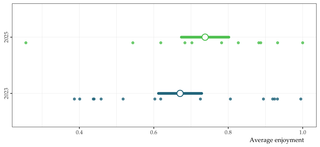

Figure 1: Average enjoyment ratings as a function of year. Transparent points represent raw data. Larger, white points represent means \(\pm\)SE.

It looks like the average difference between years is quite small. We will fit a linear model to test the hypothesis that the mean difference = 0. The inclusive model formula is enjoy ~ year.

# Fit null model
mod_q1_0 <- lm(avg_enj ~ 1, data = enjoy_avg_id)

# Fit inclusive model
mod_q1_1 <- lm(avg_enj ~ year, data = enjoy_avg_id)

# Nested model comparison
anova(mod_q1_0, mod_q1_1)

Analysis of Variance Table

Model 1: avg_enj ~ 1
Model 2: avg_enj ~ year
  Res.Df    RSS Df Sum of Sq      F Pr(>F)
1     25 1.1847                           
2     24 1.1560  1  0.028684 0.5955 0.4478

It looks like there is no evidence of a main effect of time (F(1) = 0.59, p = 0.45). Note, we didn’t really need to do the model comparison to find this though, as we could also just examine the summary of mod_q1_1:

tidy(mod_q1_1) |> 
  mutate_if(is.numeric, round, digits = 2) |> 
  kable()

Table 2: Summary of enjoyment ~ time model.

term	estimate	std.error	statistic	p.value
(Intercept)	0.67	0.06	11.83	0.00
year2025	0.07	0.09	0.77	0.45

Let’s interpret the output anyway…

The enjoyment data were analyzed using a standard linear model examining average enjoyment as a function of year. The year predictor was dummy coded with 2023 set as the baseline. During 2023, the average enjoyment was 0.67 \(\pm\) 0.05 standard errors (t = 11.83, p < 0.001), indicating that average enjoyment was not statistically equivalent to 0. For 2025, the average enjoyment increased relative to 2023 by 0.07 \(\pm\) 0.09 standard errors (t = 0.77, p = 0.45), but this difference is not statistically significant.

Let’s take a look at the model assumptions.

ds4ling::diagnosis(mod_q1_1)

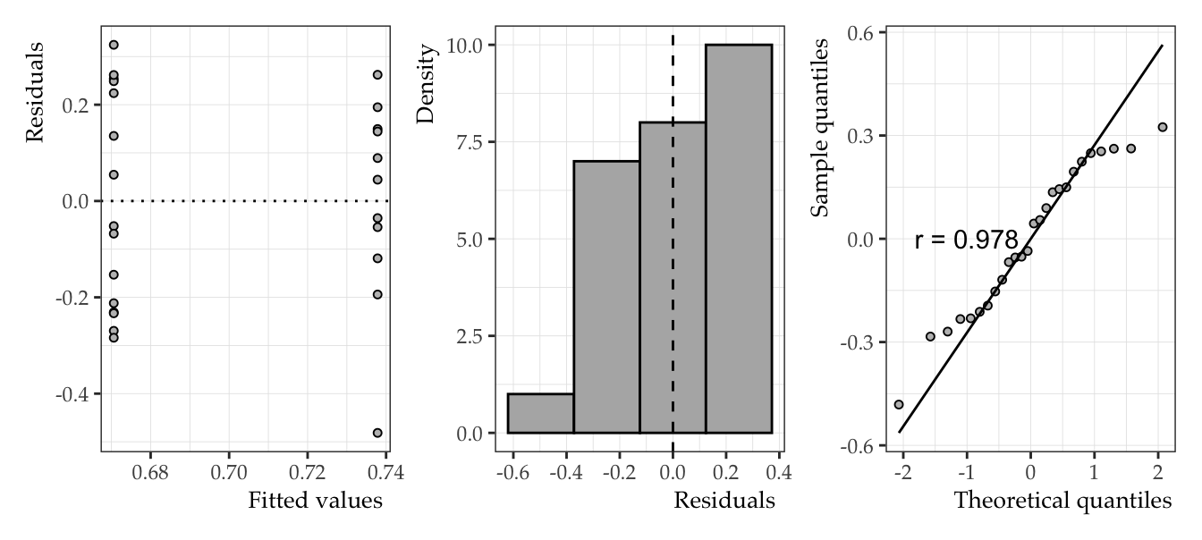
Figure 2: Residuals vs. fitted values (left panel), histrogram of residuals (middle panel), and a qq-plot (right panel) for the enjoyment (mod_q1_1) model.

It’s a bit wonky for serveral reasons. First, our only predictor is discontinuous, so the leftmost plot cannot tell us about homoscedasticity. The mean value for the residuals is essentially 0, but the distribution doesn’t not appear to be normal. Finally, we see from the qq plot that the end points don’t look great. It seems fair to assume that the residuals are not normally distributed. I probably wouldn’t put a ton of faith in this model and I think the small sample size might be an issue. A larger issue, however, has to do with the nature of the dependent variable. If we take another look at Table 1, we see that the min and max values of the enjoyment ratings range essentially from 0 to 1. This implies that, not only is the DV not normally distributed, it also does not range from -∞ to ∞. In other words, the standard linear model is not the best choice for this data set. We would be better off using a GLM with a beta likelihood and a logit linking function, i.e., beta regression. This type of distribution would be a good choice for our likelihood because it accounts for values ranging from 0 to 1 (i.e., probabilities).

Q2 - Difficulty as a function of time

Problem: Repeated measures (again).
Solution: This time we will use a multilevel model. We need to be sure that we have 1 data point per id per week. This should be the case already, but some people didn’t use the same ID every week. In other words, there is an inflated number of data points from Anonymous ID. Let’s check this out and come up with a solution.

# Get a vector of all unique IDs
dat |> 
  pull(id) |> 
  unique()

 [1] "Anon1"                "Anonymous ID2"        "Anonymous ID"        
 [4] "Catling"              "Dasani"               "Juaquín"             
 [7] "Jukun Zhang"          "Lolex"                "anon86_a"            
[10] "apricot_a"            "cervatillo silvestre" "charleshsueh"        
[13] "dusty"                "greentruck"           "jz"                  
[16] "knf43"                "lingcat"              "me"                  
[19] "mmmerlinski"          "notasuperhero"        "pear"                
[22] "sherlock_holmes"      "spiderman"            "sunflower_a"         
[25] "syntaxisscary"       

What we see here is that we have 3 anonymous-like IDs (Anon1, Anonymous ID2, and Anonymous ID). I suspect that Anonymous ID will be the only problem, but let’s check to be sure.

# Get number of data points from Anon1, AnonymousID2, and Anonymous ID
dat |> 
  filter(id %in% c("Anon1", "Anonymous ID2", "Anonymous ID")) |> 
  group_by(id) |> 
  count()

# A tibble: 3 × 2
# Groups:   id [3]
  id                n
  <chr>         <int>
1 Anon1            11
2 Anonymous ID     24
3 Anonymous ID2     1

A given participant should have a maximum of 11 data points. To simplify the problem, we will just filter out anybody with more than 11.

# Get vector of IDs with 11 or fewer data points
good_ids <- dat |> 
  group_by(id) |> 
  count() |> 
  filter(n <= 11) |> 
  pull(id)

dat_avg_time <- dat |> 
  filter(id %in% good_ids) |> 
  group_by(id, week) |> 
  summarize(difficulty = mean(difficulty), .groups = "drop") |> 
  mutate(week = week - 1) 

Now let’s take a look at how complete the data set is. I want to see how many time data points we have for each ID.

dat_avg_time |> 
  group_by(id) |> 
  count() |> 
  kable()

Table 3: Number of data points from each unique ID.

id	n
Anon1	11
Anonymous ID2	1
Catling	6
Dasani	11
Juaquín	9
Jukun Zhang	11
Lolex	9
anon86_a	2
apricot_a	2
cervatillo silvestre	8
charleshsueh	10
dusty	8
greentruck	9
jz	7
knf43	5
lingcat	1
me	8
mmmerlinski	10
notasuperhero	9
pear	7
sherlock_holmes	6
spiderman	9
sunflower_a	6
syntaxisscary	5

Table 3 shows us that we have really incomplete data. Ok. Let’s see average difficulty for each week.

dat_avg_time |> 
  group_by(week) |> 
  summarize(
    n = n(), 
    min = min(difficulty), 
    max = max(difficulty), 
    avg_difficulty = mean(difficulty), 
    sd_difficulty = sd(difficulty)
  ) |> 
  mutate(across(min:sd_difficulty, \(x) round(x, digits = 2))) |> 
  kable()

Table 4: Average difficulty as a function of week.

week	n	min	max	avg_difficulty	sd_difficulty
0	21	0.00	0.87	0.28	0.23
1	19	0.13	1.00	0.41	0.22
2	18	0.00	0.75	0.44	0.24
3	15	0.08	0.70	0.38	0.21
4	16	0.07	0.74	0.40	0.20
5	19	0.09	0.81	0.53	0.19
6	13	0.16	0.72	0.43	0.20
7	16	0.05	0.87	0.54	0.26
8	15	0.06	0.87	0.56	0.21
9	9	0.08	0.95	0.49	0.29
10	9	0.01	0.88	0.45	0.30

Nice! Let’s plot it.

dat_avg_time |> 
  ggplot() + 
  aes(x = week, y = difficulty) + 
  geom_point(aes(color = id), alpha = 0.4, show.legend = F) + 
  stat_summary(fun.data = mean_se, geom = "pointrange", pch = 21, fill = "white") + 
  scale_x_continuous(breaks = 0:10, labels = 1:11) + 
  labs(y = "Avg. difficulty rating", x = "Week") + 
  ds4ling::ds4ling_bw_theme()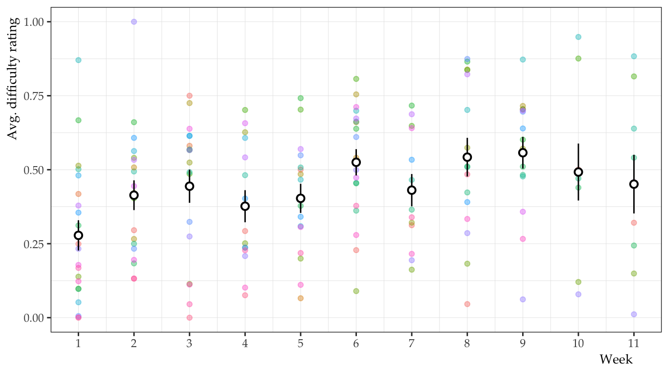

Figure 3: Average difficulty by week.

It looks like difficulty increases slightly over time, particularly if we compare week 1 to week 11. That said, the trend does not appear to be linear (we’ll come back to this). Now we can fit a multilevel model testing difficulty over time. Our inclusive model is: difficulty ~ week + (1 + time | id).

# Load multilevel model packages
library("lme4")
library("lmerTest")

# Fit nullmodel
q2_mod_0 <- lmer(difficulty ~ 1 + (1 + week | id), data = dat_avg_time)

# Fit inclusive model
q2_mod_1 <- lmer(difficulty ~ 1 + week + (1 + week | id), data = dat_avg_time)

# Nested model comparisons
anova(q2_mod_0, q2_mod_1, reml = F)

Data: dat_avg_time
Models:
q2_mod_0: difficulty ~ 1 + (1 + week | id)
q2_mod_1: difficulty ~ 1 + week + (1 + week | id)
         npar     AIC     BIC logLik -2*log(L)  Chisq Df Pr(>Chisq)   
q2_mod_0    5 -81.911 -66.232 45.955   -91.911                        
q2_mod_1    6 -88.717 -69.902 50.359  -100.717 8.8061  1   0.003002 **
---
Signif. codes:  0 '***' 0.001 '**' 0.01 '*' 0.05 '.' 0.1 ' ' 1

summary(q2_mod_1)

Linear mixed model fit by REML. t-tests use Satterthwaite's method [
lmerModLmerTest]
Formula: difficulty ~ 1 + week + (1 + week | id)
   Data: dat_avg_time

REML criterion at convergence: -87.8

Scaled residuals: 
    Min      1Q  Median      3Q     Max 
-2.4131 -0.5424 -0.0309  0.5017  3.8944 

Random effects:
 Groups   Name        Variance  Std.Dev. Corr 
 id       (Intercept) 0.0258803 0.16087       
          week        0.0007964 0.02822  -0.42
 Residual             0.0213193 0.14601       
Number of obs: 170, groups:  id, 24

Fixed effects:
             Estimate Std. Error        df t value Pr(>|t|)    
(Intercept)  0.346338   0.039250 21.129932   8.824 1.57e-08 ***
week         0.023764   0.007504 20.954441   3.167  0.00465 ** 
---
Signif. codes:  0 '***' 0.001 '**' 0.01 '*' 0.05 '.' 0.1 ' ' 1

Correlation of Fixed Effects:
     (Intr)
week -0.532

Interpretation:

The difficulty data was analyzed using a multilevel model. We fit difficulty ratings as a function of week (1-11). Week was set as a continuous predictor and was allowed to vary for each individual id. We assessed the main effect of time using a nested model comparison. There was a main effect of time (\(\chi\)(1) = 8.79, p = 0.003). At week 1, average difficulty was approximately 0.35 \(\pm\) 0.03 standard errors (t = 9.33, p < 0.001). As each week progressed the average difficulty rating increased by approximately 0.02 \(\pm\) 0.007 standard errors (t = 3.15, p = 0.004). In other words, the average perception of difficulty increased, though slightly, as the semester unfolded.

Some assumptions:
While we were able to account for the structure of the data using a multilevel model, i.e., the repeated measures week, we are still not using the best model because we have a dependent variable that is bounded between 0 and 1. We could fit a better model with beta regression (i.e., beta likelihood with logit link). Furthermore, as noted above, the relationship between difficulty rating and time does not seem to be linear (recall that this is a key assumption). This makes sense, as some content might be considered to be more or less difficult. We would probably be better off using a non-linear model, like a GAMM.

Q3 - The relationship between enjoyment and difficulty

Problem: Repeated measures (again).
Solution: Lots of averaging or use a multilevel model

Lets average to go fast. For the purposes of this question, we will forget about the effect of time. We are merely considering a global rating of enjoyment and difficult for the class.

# Calculate average enjoyment rating and average difficulty per ID
enj_diff <- dat |> 
  group_by(id) |> 
  summarize(enjoyment = mean(enjoy, na.rm = T), difficulty = mean(difficulty, na.rm = T))

head(enj_diff)

# A tibble: 6 × 3
  id            enjoyment difficulty
  <chr>             <dbl>      <dbl>
1 Anon1             0.887     0.382 
2 Anonymous ID      0.690     0.466 
3 Anonymous ID2     0.458     0.0657
4 Catling           0.895     0.631 
5 Dasani            0.544     0.644 
6 Juaquín           0.684     0.358 

Let’s make a table of some basic descriptive statistics.

enj_diff |> 
  pivot_longer(
    cols = enjoyment:difficulty, 
    names_to = "Metric", 
    values_to = "Rating"
  ) |> 
  group_by(Metric) |> 
  summarize(
    n = n(), 
    Min. = min(Rating), 
    Max. = max(Rating), 
    Average = mean(Rating), 
    SD = sd(Rating)
  ) |> 
  mutate(Metric = stringr::str_to_title(Metric)) |> 
  mutate(across(Min.:SD, \(x) round(x, digits = 2))) |> 
  kable()

Table 5: Descriptive statistics of global difficulty and enjoyment ratings.

Metric	n	Min.	Max.	Average	SD
Difficulty	25	0.07	0.78	0.43	0.17
Enjoyment	25	0.26	1.00	0.71	0.21

Ok. Table 5 gives us a good feel of the overall rating of the course. It doesn’t appear to be too difficult and the students seem to enjoy it. Win! However, this doesn’t tell us anything about the relationship between difficulty and enjoyment ratings. Let’s make a plot.

enj_diff |> 
  ggplot() + 
  aes(x = difficulty, y = enjoyment) + 
  geom_point() + 
  geom_smooth(method = "lm", formula = "y ~ x") + 
  labs(y = "Avg. enjoyment rating", x = "Avg. difficulty rating") + 
  ds4ling::ds4ling_bw_theme()

Figure 4: Scatter plot of global enjoyment and difficulty ratings from 2023 and 2025.

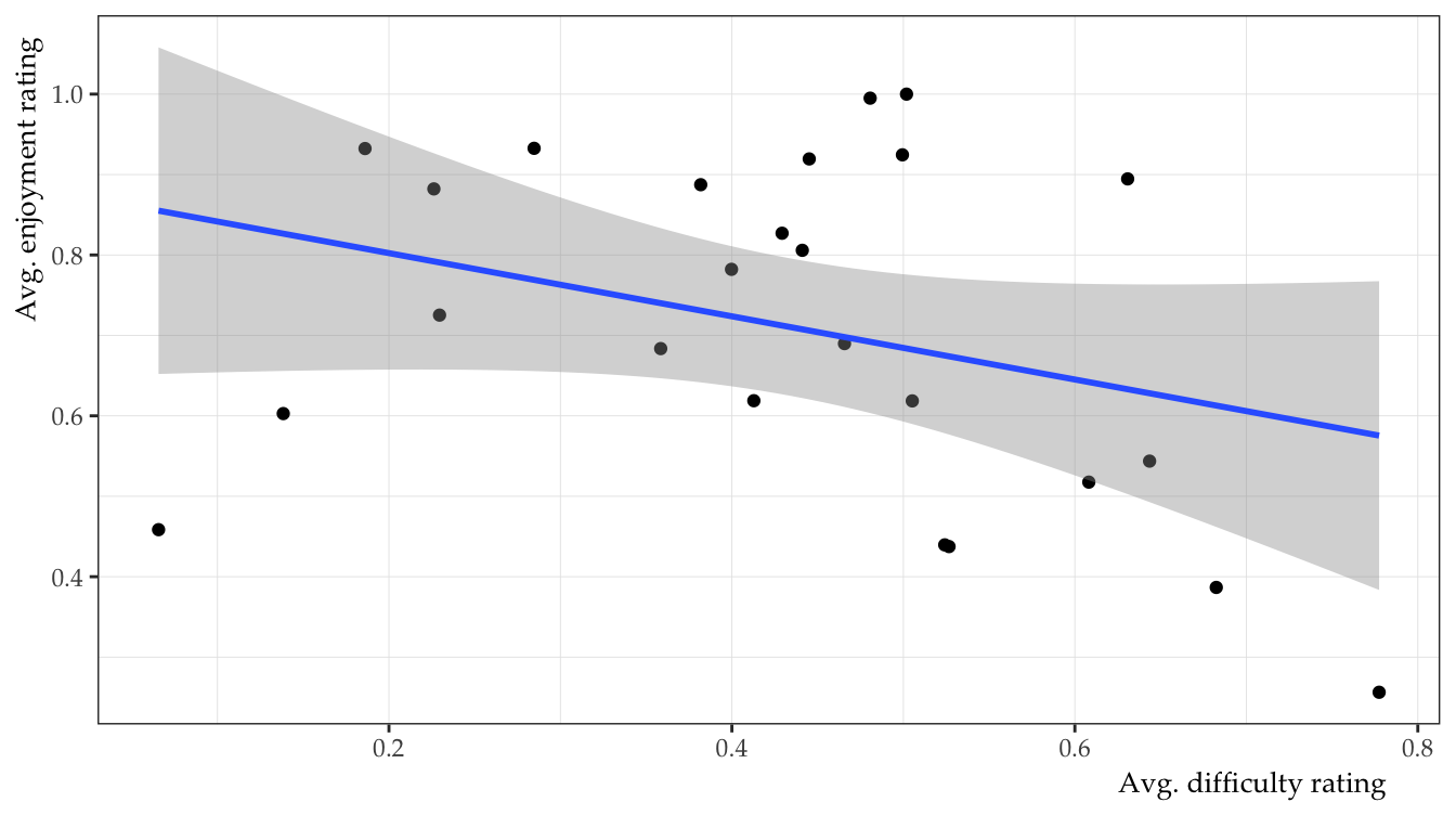
The quick and dirty plot suggests a negative correlation between enjoyment and difficulty. In other words, people might enjoy class less when the content is difficult. We will test this hypothesis with a standard linear model. We don’t really need any nested model comparisons here, but we will do it for the sake of completeness.

# Fit null model
q3_mod_0 <- lm(enjoyment ~ 1, data = enj_diff)

# Fit inclusive model
q3_mod_1 <- lm(enjoyment ~ difficulty, data = enj_diff)

# Nusted model comparison
anova(q3_mod_0, q3_mod_1)

Analysis of Variance Table

Model 1: enjoyment ~ 1
Model 2: enjoyment ~ difficulty
  Res.Df     RSS Df Sum of Sq      F Pr(>F)
1     24 1.09266                           
2     23 0.98022  1   0.11244 2.6383 0.1179

tidy(q3_mod_1) |> 
  mutate_if(is.numeric, round, digits = 2) |> 
  kable()

Table 6: Summary of enjoyment ~ time model.

term	estimate	std.error	statistic	p.value
(Intercept)	0.88	0.11	7.81	0.00
difficulty	-0.39	0.24	-1.62	0.12

Interpretation:

When difficulty is 0, enjoyment is high (\(\beta\) = 0.88, SE = 0.11, t = 7.81, p < 0.001). A one unit increase in difficulty results in a decrease in enjoyment, but the relationship is not statistically significant (\(\beta\) = -0.39, SE = 0.24, t = -1.62, p = 0.12).

Aside from the other caveats (beta regression for DV), it is of note that we are certainly losing a lot of power by averaging over time. A multilevel model would probably make more sense for this data.