Data Science for Linguists
The linear model: Multiple regression
Joseph V. Casillas, PhD
Rutgers University
Last update: 2025-03-22
Multiple regression and correlation
MRC
Multiple Causation
- In nature: a phenomenon may have more than a single cause
- In statistics: criterion variable might have more than a single relevant predictor
- Leaving a potential cause out of the equation would constitute “omitting a relevant variable”
- This biases the parameter estimates for the other predictors
- We are not always sure of what those other predictors might be!
MRC
Overview
- We have specified a linear formula that can account for the relationship between two continuous variables.
\[Y = a + bX + e\]
- It is uncommon for a given response variable to be determined by a single predictor
- Most theories/models in social science predict complex relationships between multiple predictors.
- Score ~ SES + IQ
- Duration ~ speech rate + number of syllables
- RT ~ working memory + word position
- We can extend the linear model equation to account for multiple predictors.
MRC
Overview
- We want to construct the equivalent of an OR statement or a logical disjunction
- Boolean Algebra tells us that an OR statement implies summing things
- In other words, all X’s do not have to be high at once to have an effect on Y
- For example, you can get an overall high GRE score by scoring high in verbal but (somewhat) low in math:
- They have to have a high total (or sum)
- A sum is implicitly an OR statement
| A (x) |
B (y) |
C (x ∨ y) |
|---|---|---|
| 0 | 0 | 0 |
| 0 | 1 | 1 |
| 1 | 0 | 1 |
| 1 | 1 | 1 |
OR
B = 1,
then C = 1
Otherwise, C = 0
MRC
Overview
- What if we based linguistics Grad School
acceptances solely on GRE scores?
- One shouldn’t have to score high on all of
the entrance requirements, but just rank
high on the sum of all of them
- We could use a weighted sum
MRC
Overview
Weighted sum
- Some things are more important than others in this overall sum
- For example, GRE is actually a poor predictor of graduate student success
- So we might want to weight this variable lower than something like GPA or letters of recommendation
- We can use least squares estimation to get the b-weights with the lowest SSERROR
MRC
The equation
\[Y = a + bX + e\]
\[Y = a_{0} + b_{1}X_{1} + b_{2}X_{2} {...} b_{k}X_{k} + e\]
Least Squares Estimation
- R will estimate the b-weights that minimize the sum of the squared errors (🙅 by hand examples)
- Ideally these are the b-weights that best represent how much each predictor is really contributing to the variance in the criterion variable (y)
- We will again use least squares estimation to achieve the best (optimal) regression weights
MRC
Multiple predictors
- The multiple predictors represent different hypotheses regarding what might be affecting the criterion variable
- In other words, multiple regression is just creating a sum of weighted predictors to explain the total variance in the criterion variable
- The way that the predictors function together is not necessarily the same as the way that they each function alone
- Bivariate regression is just a degenerate form (“special case”) of multiple regression containing only one predictor
MRC
Interpretation
Summarizing so far…
- In multiple regression we assume additivity and linearity
- In Boolean Algebra, a sum (addition) represents a logical disjunction
- The multiple regression “weighted sum” is a complex OR statement
What does this mean for our parameter estimates and how do we interpret them?
MRC
(Semi)partial betas
- Intercept ( \(a_{0}\) ): the value of the criterion variable when all predictors are equal to 0 (same as bivariate regression)
- Slope ( \(b_{k}\) ): the change in the criterion associated with a 1-unit change in \(X_k\)… with all other predictors held constant
How can we calculate the unique contribution of each predictor?
MRC
MRC
Recall that the b-weight
of the bivariate model is \(r(\frac{s_y}{s_x})\)
MRC
MRC
The “Ballantine”
Cohen & Cohen (1975)
MRC
- \(r^{2}_{x1,x2} = c + d\)
- \(r^{2}_{y,x1} = a + c\)
- \(r^{2}_{y,x2} = b + c\)
- \(R^{2}_{y,x1,x2} = a + b + c\)
MRC
Squared semipartial correlation
- \(X_2\) removed from explained
variance - Represents unique contribution
of \(X_1\) - \(sr^2 = R^{2}_{y,x1,x2} - r^{2}_{y,x2}\)
MRC
Squared partial
correlation
- Y variance not accounted for by
\(X_2\) is the area of A + E - The area explained by \(X_1\) = A
(squared semipartial correlation) - Unqiue contribution of \(X_1\) is
\(A / (A + E)\) or… - \(pr^{2}_{x1} = \frac{A}{A + E}\)
- We are pretending that \(X_2\)
doesn’t exist (statistically)
MRC
Statistical control1
- Not the same as experimental control
- We are interested in some treatment
- Some participants receive treatment, some do not
- Only looking at highly proficient bilinguals (not low, med. prof.)
- We partial out the effects of predictor \(X_1\) from all other predictors and use this error to determine \(b_1\)
- We are estimating the effect of one predictor while holding the other predictors constant
- This will only work if predictors are not correlated (i.e., there cannot be multicollinearity)
MRC
Conceptual understanding
- MRC is much more difficult to conceptualize than the bivariate linear regression
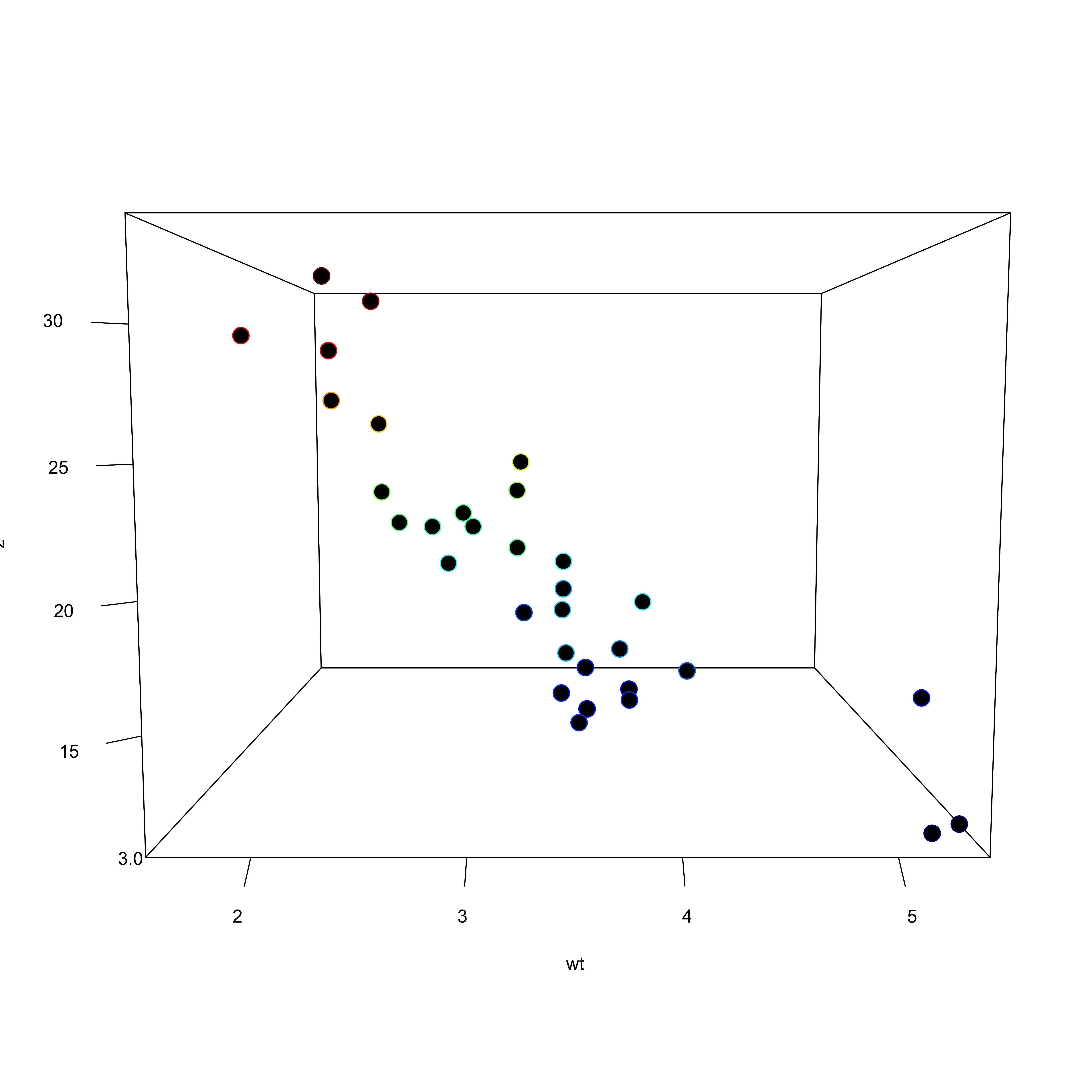
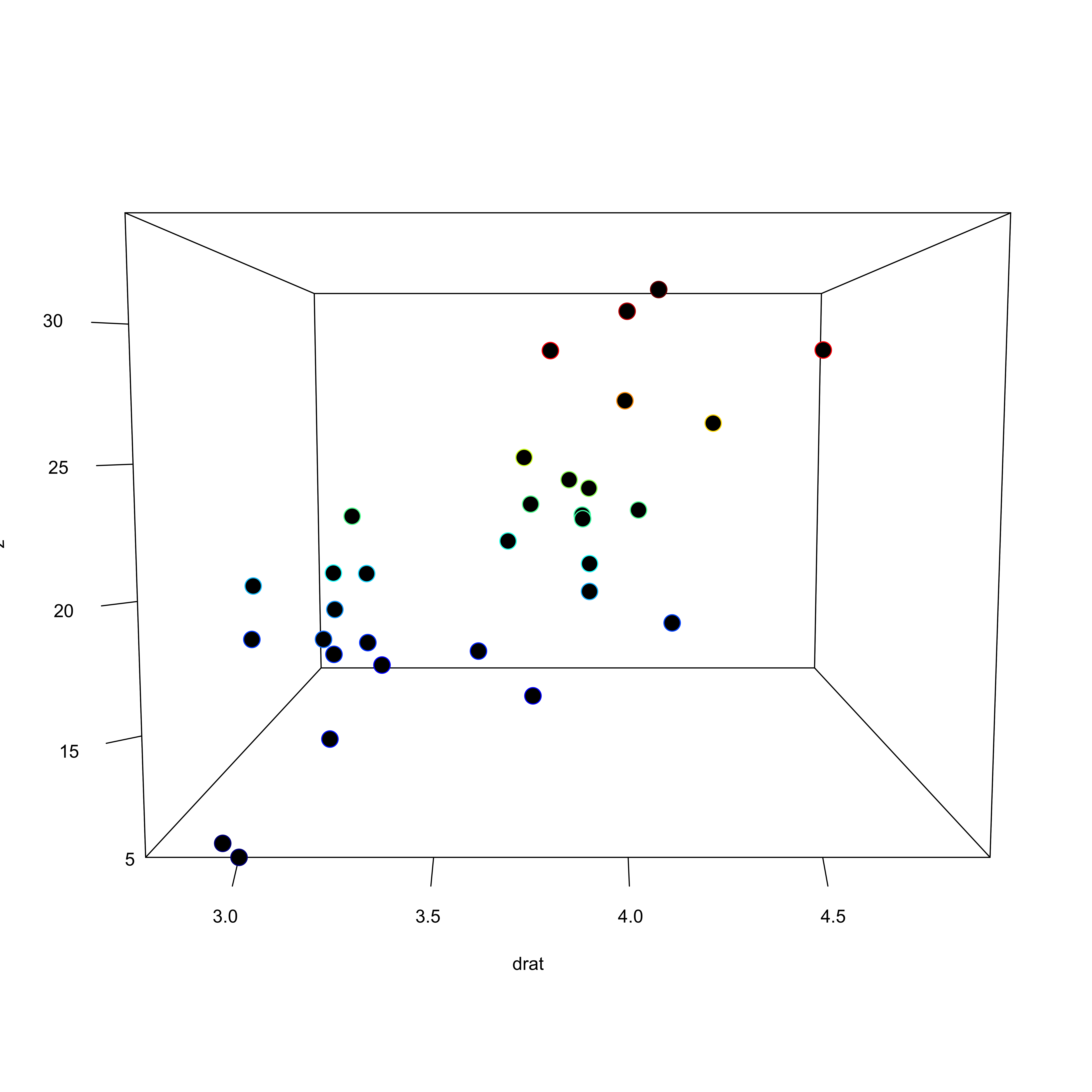
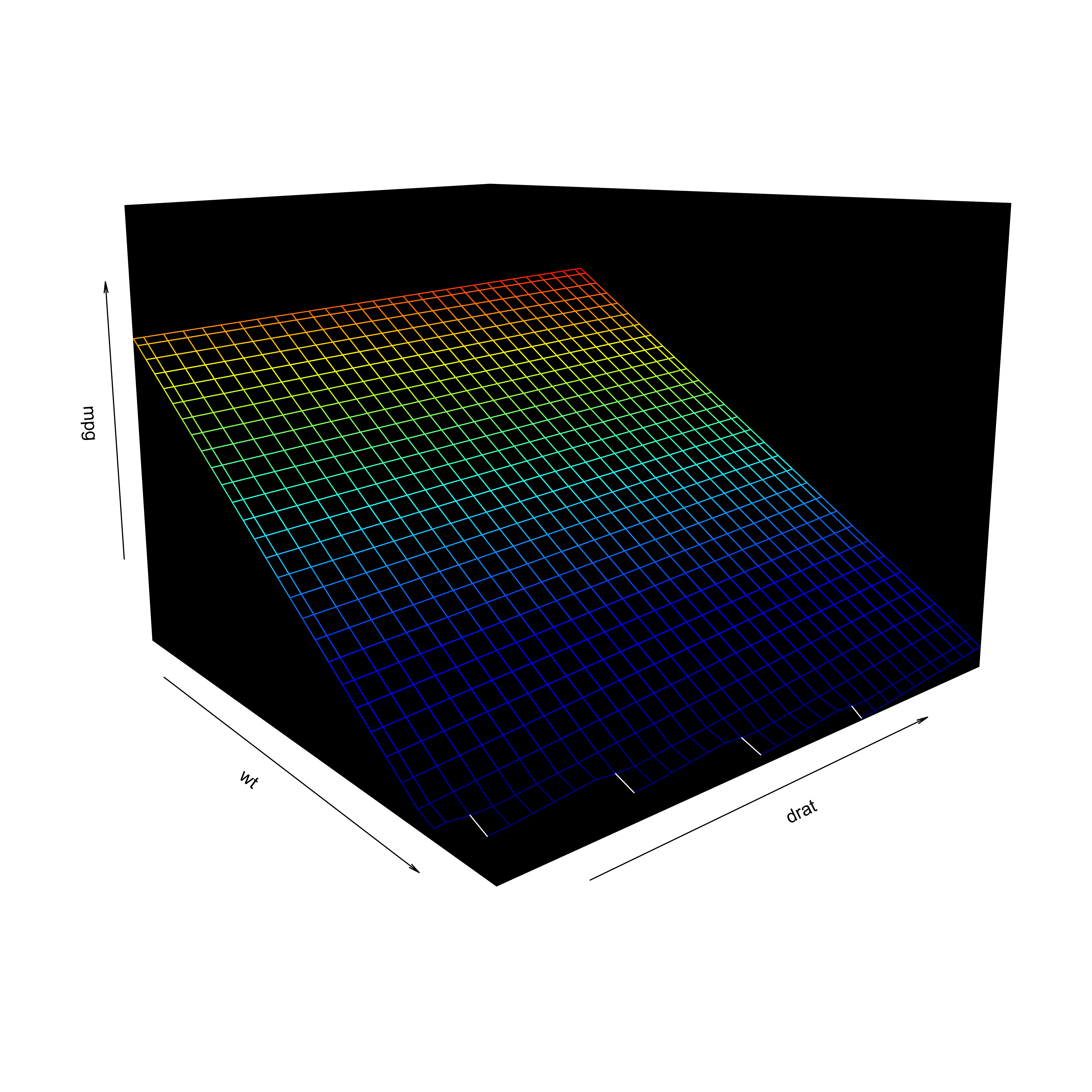
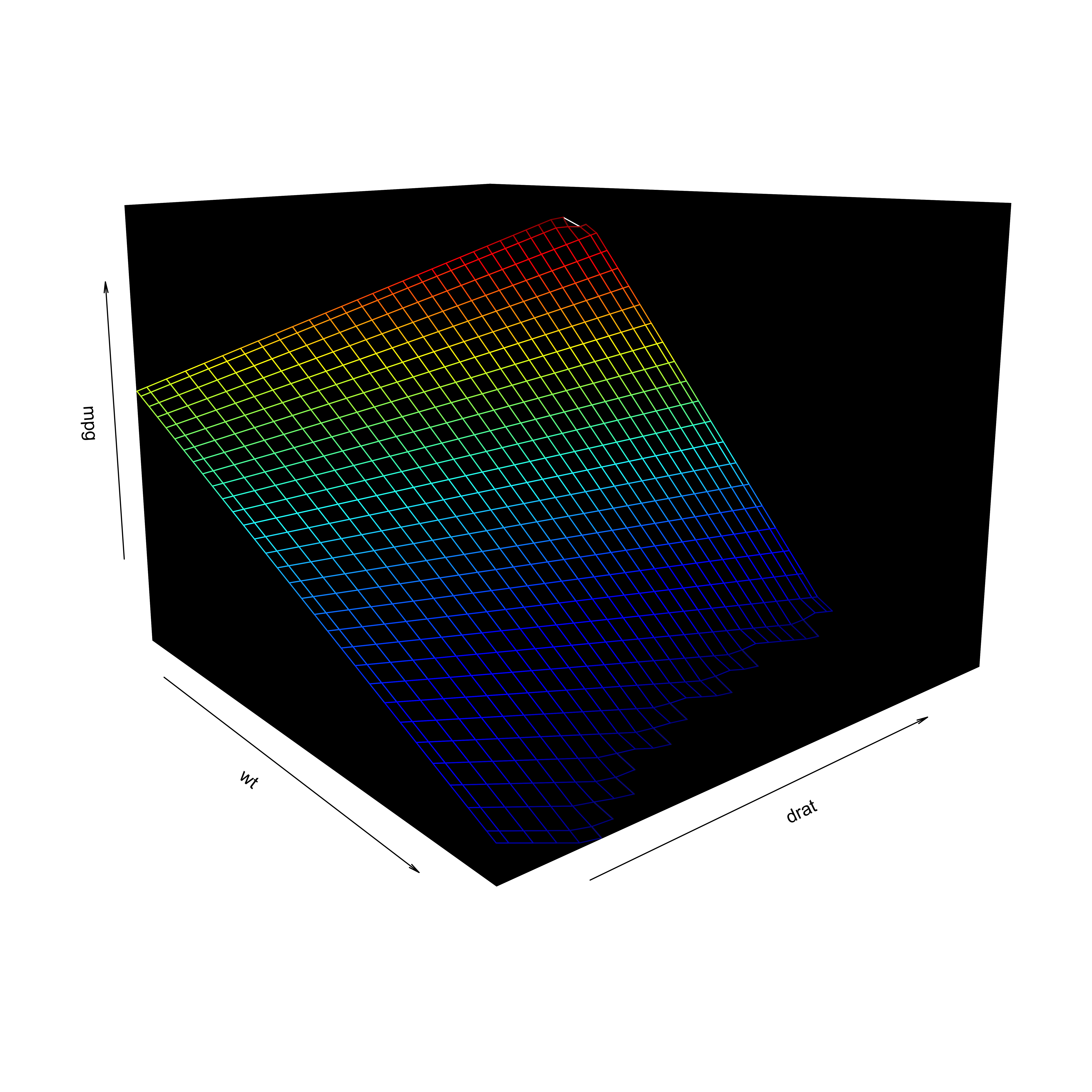
- If we consider a simple three variable model (y ~ x1 + x2) we are fitting a hyperplane to a three dimensional space
- More variables = more complexity
MRC
!=
MRC
MRC
MRC

MRC
MRC
Doing it in R
Call:
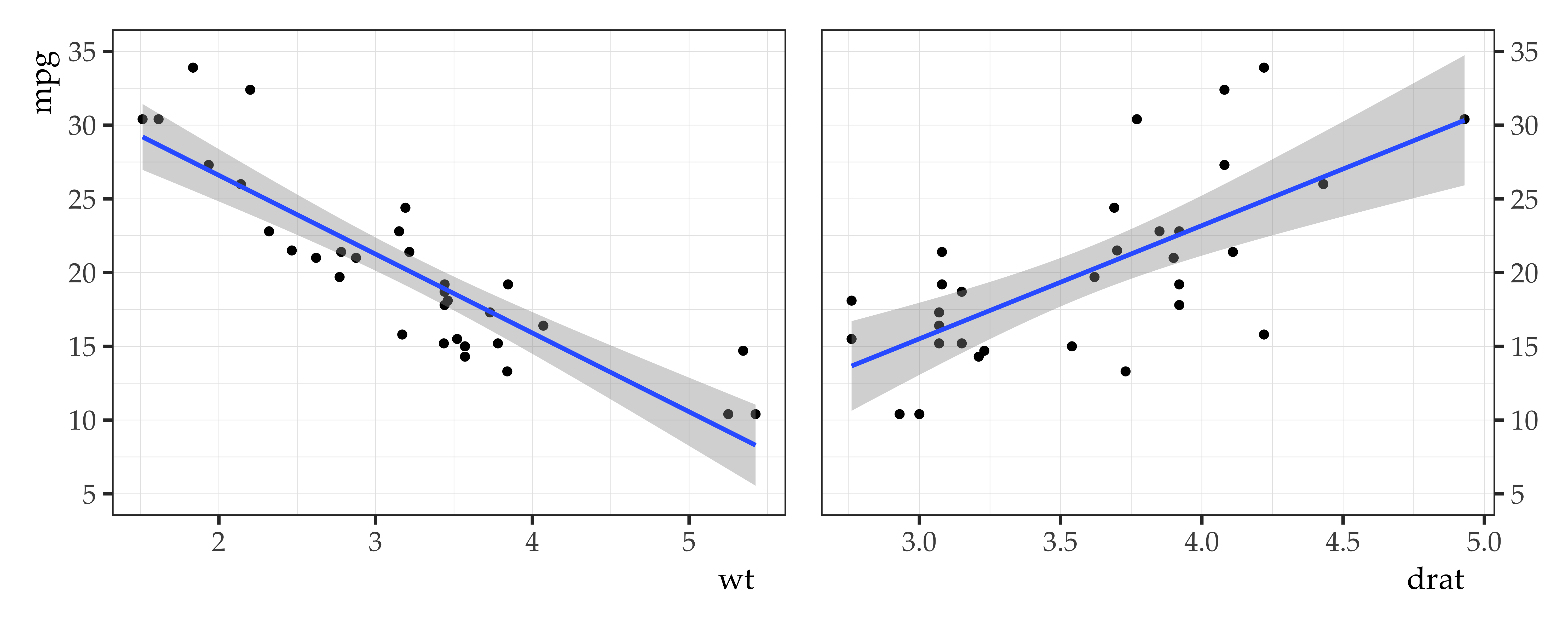
lm(formula = mpg ~ wt + drat, data = mtcars)
Residuals:
Min 1Q Median 3Q Max
-5.4159 -2.0452 0.0136 1.7704 6.7466
Coefficients:
Estimate Std. Error t value Pr(>|t|)
(Intercept) 30.290 7.318 4.139 0.000274 ***
wt -4.783 0.797 -6.001 1.59e-06 ***
drat 1.442 1.459 0.989 0.330854
---
Signif. codes: 0 '***' 0.001 '**' 0.01 '*' 0.05 '.' 0.1 ' ' 1
Residual standard error: 3.047 on 29 degrees of freedom
Multiple R-squared: 0.7609, Adjusted R-squared: 0.7444
F-statistic: 46.14 on 2 and 29 DF, p-value: 9.761e-10MRC
CIs and significance tests
| beta | SE | 95% LB | 95% UB | t-ratio | p.value | |
|---|---|---|---|---|---|---|
| (Intercept) | 30.29 | 7.32 | 15.32 | 45.26 | 4.14 | 0.00 |
| wt | -4.78 | 0.80 | -6.41 | -3.15 | -6.00 | 0.00 |
| drat | 1.44 | 1.46 | -1.54 | 4.43 | 0.99 | 0.33 |
- Same as bivariate case, but we adjust t-value for k (added estimated parameters)
- Statistical significance implies that the 95% CI doesn’t contain 0
- Rule of thumb: multiply SE of b-weight by 2 and add/subtract to/from b-weight
- T-ratio: Parameter estimate divided by SE
(i.e., 30.29 / 7.32 = 4.14) - Rule of thumb: |t| > 2 = significant™
MRC
Coefficient of multiple determination: R2
- Adding variables will always explain more variance
- Not necessarily better
- There is an adjustment for exhausting degrees of freedom
Note
- r: pearson product moment correlation
- r2: coefficient of determination; variance explained (bivariate case)
- R2: coefficient of multiple determination; variance explained (MRC)
MRC
Making predictions
- Recall the multiple regression equation…
\[Y = a_{0} + b_{1}X_{1} + b_{2}X_{2} {...} b_{k}X_{k} + e\]
- Our
mtcarsmodel can be summarized as…
\[ \begin{aligned} \widehat{mpg} &= 30.29 + -4.78(wt) + 1.44(drat) \end{aligned} \]
What is the predicted mpg for a car that weighs 1 unit with a rear axel ratio (drat) of 2?
And one that weighs 1 with a drat of 4?
And one that weighs 3 with a drat of 2.5?
- 28.39 \(mpg = 30.29 + -4.78 \times 1 + 1.44 \times 2\)
- 31.28 \(mpg = 30.29 + -4.78 \times 1 + 1.44 \times 4\)
- 19.55 \(mpg = 30.29 + -4.78 \times 3 + 1.44 \times 2.5\)
Interactions
Interactions
Recall
- Assumptions of Multiple Regression:
- Additivity
- Linearity
- In Boolean Algebra, a sum (addition) represents a logical disjunction:
- Multiple regression “weighted sum” is a complex “OR” statement
| A (x) |
B (y) |
C (x ∨ y) |
|---|---|---|
| 0 | 0 | 0 |
| 0 | 1 | 1 |
| 1 | 0 | 1 |
| 1 | 1 | 1 |
If A = 1
OR
B = 1,
then C = 1
Otherwise, C = 0
Interactions
Recall
- Assumptions of Multiple Regression:
- Additivity
- Linearity
- In Boolean Algebra, a sum (addition) represents a logical disjunction:
- Multiple regression “weighted sum” is a complex “OR” statement
Non-Additivity: Interaction Terms
- In Boolean Algebra, a product (multiplication) represents a logical conjunction:
- Interaction terms represent “AND” terms
- These are included within the overall “OR” statement
| A (x) |
B (y) |
C (x ∧ y) |
(x ∨ y) |
|---|---|---|---|
| 0 | 0 | 0 | 0 |
| 0 | 1 | 0 | 1 |
| 1 | 0 | 0 | 1 |
| 1 | 1 | 1 | 1 |
If A = 1
AND
B = 1,
then C = 1
Otherwise, C = 0
Interactions
Genetics example
- You share 50% of genes with your Mom (M) and 50% with your Dad (D)
- But your parents don’t share that many genes
- M and D are generally not genetically correlated with each other, but you (the M*D interaction) are correlated with both M and D (more on this later)
Drugs and alcohol
Consider taking the upcoming midterm in one of the following conditions
- Neither Drugs nor Alcohol:
- probably best, produce highest score
- Alcohol alone:
- Probably lower midterm scores than doing neither
- Drugs alone:
- Probably lower midterm scores than doing neither
- Alcohol and Drugs together:
- Probably lowest scores on the midterm exam of all the four possible conditions
Interactions
Drugs and alcohol continued
- Is the effect of alcohol and drugs together equal to the negative effect of alcohol PLUS the negative effect of drugs?
- Probably not
- Alcohol and drugs are known to interact
- This effect is a negative interaction
- If you mix alcohol and drugs they have a larger combined effect than adding up the effects of each acting separately:
- For example, if alcohol makes your score drop 10 points, and the drug drops it 15 points, when you take both your score will very likely drop more than just 25 points
- This effect is not additive, it is multiplicative
Interactions
Non-additivity of effects
- You cannot add the effect of alcohol to the effect of drugs to predict the effect “alcohol AND drugs”
- Because you get an extra effect (a boosting effect) by combing them
- There is a synergistic effect of combining the terms
- In principle, could be either more or less effective
- You include this multiplicative AND term (A*D) in ADDITION to the other terms in the model
Interactions
The multiple regression formula:
\(Y = a_{0} + b_{1}X_{1} + b_{2}X_{2} + (b_{1}X_{1} \times b_{2}X_{2}) + e\)
Including interactions in R
- We do this using :
- Or *
Call:
lm(formula = mpg ~ wt + drat + wt:drat, data = mtcars)

Residuals:
    Min      1Q  Median      3Q     Max
-3.8913 -1.8634 -0.3398  1.3247  6.4730

Coefficients:
            Estimate Std. Error t value Pr(>|t|)
(Intercept)    5.550     12.631   0.439   0.6637
wt             3.884      3.798   1.023   0.3153
drat           8.494      3.321   2.557   0.0162 *
wt:drat       -2.543      1.093  -2.327   0.0274 *
---
Signif. codes:  0 '***' 0.001 '**' 0.01 '*' 0.05 '.' 0.1 ' ' 1

Residual standard error: 2.839 on 28 degrees of freedom
Multiple R-squared:  0.7996,    Adjusted R-squared:  0.7782
F-statistic: 37.25 on 3 and 28 DF,  p-value: 6.567e-10
Interactions
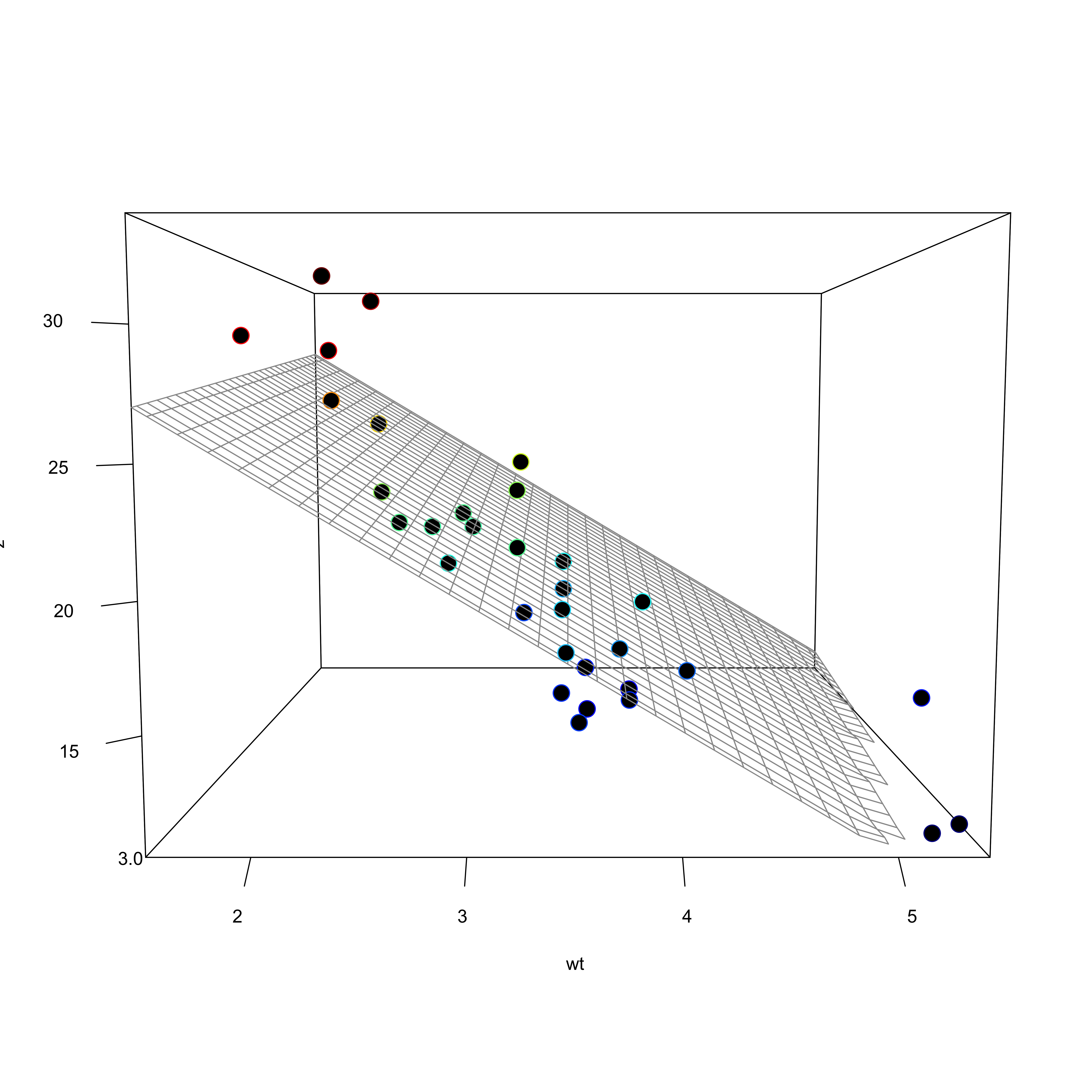
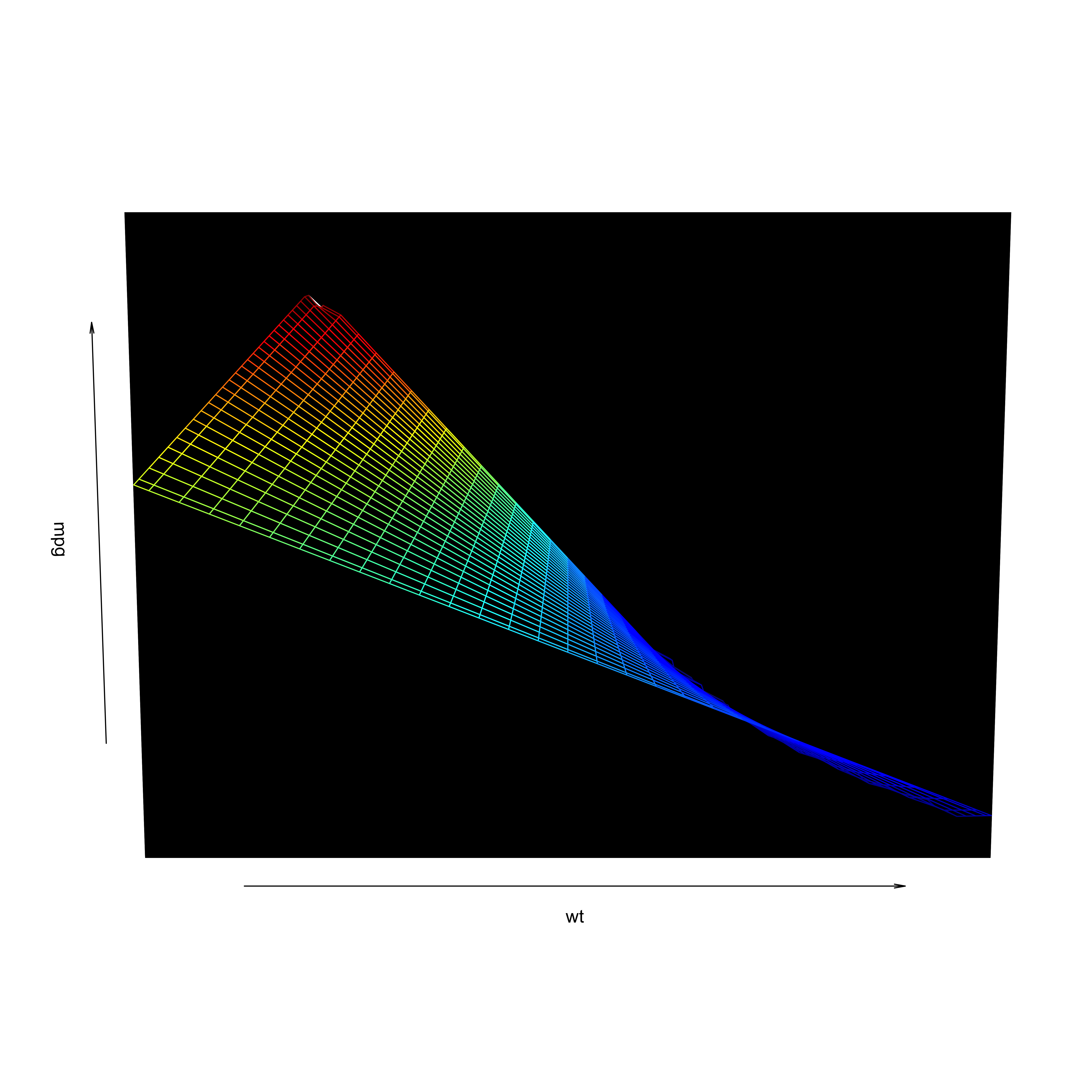
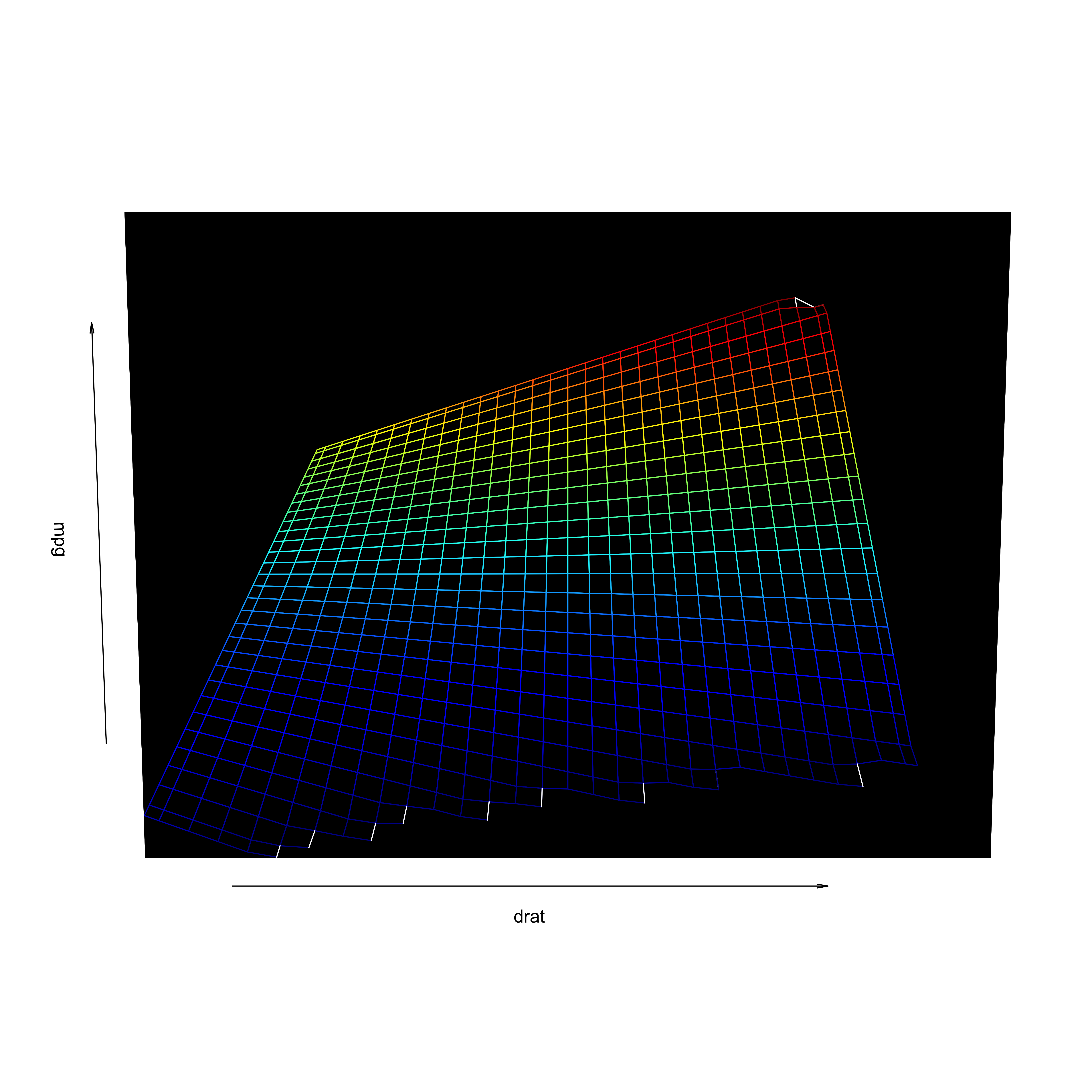
Visualization
- Including an interaction affects the hyperplane fit to the data
Interactions


Interactions
Interactions


Interactions
Review
What we’ve seen so far
- Bivariate regression
- MRC
- Additive effects
- Interactions
(multiplicative effects)
What’s left
- Assumptions
- Model specification
- Alpha slippage
- Empirical selection of variables
- Reporting results
Assumptions
(revisited)
A new assumption
Multicollinearity
- Multicollinearity occurs when the predictors are correlated
- height (x1) and weight (x2)
- intelligence (x1) and creativity (x2)
A new assumption
Multicollinearity
- Why is it a problem?
- “Confounds” produce ambiguity of causal inference
- Least Squares Estimation in Linear Model:
- Simultaneous estimation of additive effects of all model predictors
- Does not adequately partition variance among correlated predictors
- Least squares estimation is not adequate for dealing with multicollinearity
- works best when predictors are uncorrelated
Old assumptions revisited
Model specification errors
Avoid excluding relevant variables
- Use Multiple Working Hypotheses
- This is how you safeguard against leaving out a variable that you might need later
- But don’t put in everything but the kitchen sink…you also must avoid including irrelevant variables
- Ideally you want to use plausible rival hypotheses
- You need to have some theory behind your reasoning
- Assuming you have done all of this, we need to figure out which predictors are relevant and which are not relevant
- This is not nearly as a big of a problem as having excluded a relevant variable
How useful is the model output?
Traditional t-test to determine if the b = 0
- Take b-weight, compute standard error
- Use SEb and the b-weight and construct a t-ratio:
\[t_{b} = \frac{b}{SE_{b}}\]
- Theoretically this informs us of whether b = 0 or not
Problem
- The b-weights and the SE of the b-weight are both critically dependent on the model being correctly specified!
- If you made either kind of model specification error, the parameter estimates are invalid
- The b-weights might have changed if you omitted a relevant variable
- The SE of the b-weights will have changed (increased) if you included an irrelevant variable
How useful is the model output?
Your t-tests might not be informative
- If the model is not correctly specified then it is based on incorrect values of either b or SEb or both
- If you knew the model was correctly specified then you would have no need to use the t-tests in the first place
- You only need to use them if you’re unsure whether the model is correctly specified
- So the only conditions in which the tests are useful are the conditions in which they may be invalid!
- But you only test this if you are questioning the specification of the model
How do you deal with this?
Hierarchical partitioning of variance through nested model comparisons
Hierarchical Partitioning of Variance
Hierarchical Partitioning of Variance
Nested model comparisons
- Comparison of “hierarchically nested” multiple regression models
- Requires theoretical specification and causal ordering of predictors
Nested model comparisons
What is a nested model?
A nested model is when one model is nested inside the other such that there is a more inclusive model that contains more parameters and a less inclusive model (restricted model) that contains just a subset of specific variables you would like to test
Nested model comparisons
What is a nested model?
- In nested model comparisons, you are testing whether those parameters not in the restricted model can be eliminated:
- You want to see if those parameters not in the restricted models can be set to 0
- You want to see if these extra parameters are needed or if they can be taken out
How
- Test a more complicated model and then a less complicated one
Nested model comparisons
Comparing nested models
- You often cannot compare two different restricted models directly
- If the models do not overlap they cannot be directly compared
- You must construct an inclusive model such that both restricted models are nested within a common inclusive model
- Then, to do the nested model comparisons you run the alternative restricted models and test each against the same inclusive model
Nested model comparisons
The semipartial R2
- The sr2 doesn’t tell you if the predictor in question is statistically significant, but rather how to estimate the unique contributions of each variable
- We are attempting the elimination of irrelevant variables with this procedure:
- We cannot address omission of a relevant variable this way (or in any other mathematical way because you cannot do math on variables that you didn’t measure in first place 🤦♀️)
- This method corrects Type I Errors only
Nested model comparisons
Inclusive Regression Model (R2I):
\[\hat{y} = a + b_{1}x_{1} + b_{2}x_{2} + b_{3}x_{3} + e\]
Restricted Regression Model (R2R):
\[\hat{y} = a + b_{1}x_{1} + b_{2}x_{2} + e\]
Nested Model Comparison:
\[(R^2_{I} - R^2_{R}) = sr^2(y, x_{3} \times x_{1}, x_{2})\]
Nested model comparisons: (kI - kR) = 1
Restricted Regression Model 1:
\[\hat{y} = a + b_{1}x_{1} + b_{2}x_{2} + e\]
Restricted Regression Model 2:
\[\hat{y} = a + b_{1}x_{1} + b_{3}x_{3} + e\]
Restricted Regression Model 3:
\[\hat{y} = a + b_{2}x_{2} + b_{3}x_{3} + e\]
Nested model comparisons: (kI - kR) = 2
Restricted Regression Model 4:
\[\hat{y} = a + b_{1}x_{1} + e\]
Restricted Regression Model 5:
\[\hat{y} = a + b_{2}x_{2} + e\]
Restricted Regression Model 6:
\[\hat{y} = a + b_{3}x_{3} + e\]
Nested model comparisons
How do we test semipartials?
- We will use a modification of the F-ratio (systematic variance over the error variance)
- F-ratio for sr2 = the F-ratio for the hierarchical partitioning of variance using nested model comparisons
- The sr2 of the variable of interest goes in the numerator
- The residual of the inclusive model goes in the denominator
Nested model comparisons
The semipartial F-Ratio
- This F-ratio is used like a “backward” traditional F-ratio:
- It is a test of what you have eliminated to see if you can safely eliminate it
- You only eliminate variables if doing so does not result in a significant loss of explanatory power
- It is not a test of whether what you have included is relevant:
- It’s not what’s left in the model that is being tested
- It’s what’s not in the restrictive model that is being tested
Statistics of love example
- Imagine that you have a romantic partner that you are thinking of dumping
- It might be worthwhile to see if it is a good idea by doing the math first
- So you consider what your life is like with your partner (inclusive model) and subtract what it would be like without your partner (restricted model)
- If the answer is greater than zero, you might want to retain your partner
- If it is less than or equal to zero, you may safely dump your partner
Stop voicing example
- Imagine you are looking at how skewness (x1) and kurtosis (x2) of coronal stop bursts can predict voice-onset time (y)
- You want to see if you can eliminate the kurtosis (x2) variable
- Your restricted model would be R2 (y, x1) i.e., predicting VOT from skewness alone
- If the semipartial F-ratio is not statistically significant, then you can eliminate the kurtosis variable from the model
- If the F-ratio is significant, then you cannot eliminate that variable from the model
Stop voicing example (cont)
- Suppose skewness and kurtosis can predict 40% of the variance in VOT
- If skewness alone can predict 38% of this, then:
- The squared semipartial correlation of kurtosis is 40% - 38% = 2%
- Which is less than our total error variance because 1 - 40% = 60%
- Then skewness does just fine on its own predicting VOT and we can eliminate kurtosis as a predictor
- Provided the F-ratio for the semipartial of kurtosis is not statistically significant
- This also may depend on sample size
Stop voicing example (cont)
- On the other hand, if skewness only accounts for say 10% of the variance
- Then 40% - 10% = 30%
- Then kurtosis might still be important and we cannot eliminate it from the model due to a statistically significant semipartial F-ratio
- You are testing to see if skewness is strong enough to account for VOT in coronal stops without considering kurtosis
- You want a non-significant semipartial F- ratio if you want to eliminate any variable
Nested model comparisons
Hierarchical tests of significance
\[F_{(\color{red}{k_{I}}-\color{blue}{k_{R}}),(n - \color{red}{k_{I}} - 1)} = \frac{(\color{red}{R^2_{I}} - \color{blue}{R^2_{R}}) / (\color{red}{k_{I}} - \color{blue}{k_{R}})}{(1 - \color{red}{R^2_{I}}) / (n - \color{red}{k_{I}} - 1)}\]
- R2 = Squared multiple correlation
- k = Model degrees of freedom (number of predictors)
- n = Total sample size
- I = Inclusive Model (Including All Predictors)
- R = Restricted Model (Excluding Some Predictors)
- (R2I – R2R) = Squared Semipartial Correlation
Nested model comparisons
- Results of hierarchical partitioning of variance and hierarchical tests of significance depend critically upon causal order specified among predictors:
- There is no purely mathematical solution to this problem
- Causal ordering of predictors must be specified by theory
- Comparisons of hierarchically nested models permit testing of alternative hypotheses generated by rival causal theories
- A “confound” is just an alternative hypothesis towards which one has a negative attitude
What about likelihood ratio tests?
Nested model comparisons
Genetics example revisited
- You share 50% of genes with your Mom (M) and 50% with your Dad (D)
- But your parents don’t share that many genes
- M and D are generally not genetically correlated with each other, but you (the M*D interaction) are correlated with both M and D
- So M and D are main (additive) effects and you are the M*D (multiplicative) interaction
- You are now correlated with both main effects
- This causes multicollinearity
- M and D may then argue over this shared variance
- You have become a confound
Nested model comparisons
Dealing with multicollinearity
- To test for the statistical significance of the interaction effect we use hierarchically nested model comparisons:
- This is a reasonable solution for the problem of multicollinearity
- Interaction terms (nonadditivity) ALWAYS create multicollinearity
- If the main effects are already correlated, the multicollinearity is worse:
- But you still get multicollinearity even if the component main effects are not correlated
- The purely additive model (main effects only) is simpler than the multiplicative model (including the interaction):
- So if additive model is good enough then go with it (more parsimonious)
- Leave out (eliminate) interaction effects first because they might be too confusing
Nested model comparisons
Example: A multiple regression with three predictors
y ~ a * b * c
Main effects: a, b, and c
2-way interactions: a:b, a:c, and b:c
3-way interactions: a:b:c
- Which terms get causal priority in the hierarchical partitioning of variance?
- Main effects, then 2-way interactions, then 3-way interactions, etc.
It is more parsimonious to use the main effects:
- Fewer dfs are used and it is a less complicated model
- Using a linear additive model is generally the most parsimonious way to go
- Common variance should be given first to the main effects because they are conceptually more parsimonious
Nested model comparisons
Lack of parsimony
- If you use an interaction term (e.g., a*b), you are claiming that you need BOTH in order to have an effect
- This is an extra substantive claim which needs to be supported
- It’s an AND statement not an OR statement, so it’s a bit riskier
- Inclusive model contains all interactions that you wish to test:
- Then you use restricted models to test each interaction separately
- You can generate a ridiculous amount of hypotheses with a small number of variables and this might really compromise your model parsimony:
- You need a theoretical reason to include an interaction term
Nested model comparisons
Summarizing
Problem: Multicollinearity
Solution: Hierarchical partitioning of variance
Make an inclusive model and do hierarchical partitioning of variance
Determine which terms (lower order and higher order, additive and interactive), if any, can be eliminated
Nested model comparisons
Causal priority
So which one gets causal priority?
Main effects generally do:
- But now two-way interactions and squared terms are just as complicated
- So are three-way interactions and cubed terms, etc.
There is no convention for deciding which comes first:
- There is no mathematical solution to this problem
- We need a theoretical solution
Nested model comparisons
Use principles of strong inference
Only test plausible rival hypotheses
Be careful and selective!
Even with a small number of primitive component terms (main effects), once you examine all the possible interactions you will have a complex model
You will exhaust your statistical power very quickly
Nested model comparisons
Doing it in R
- Fit all the relevant models
mod_full <- lm(mpg ~ wt + drat + wt:drat, data = mtcars) # inclusive model
mod_int  <- lm(mpg ~ wt + drat          , data = mtcars) # restricted model
mod_drat <- lm(mpg ~ wt                 , data = mtcars) # restricted model
mod_wt   <- lm(mpg ~ drat               , data = mtcars) # restricted model
mod_null <- lm(mpg ~ 1 , data = mtcars) # null model- Test higher order variables and main effects using nested model comparisons
- In R we do this with the
anova()function - It is not an anova (for that we use the
aov()function) - We include the restricted model and the inclusive model to test if removing the variable from the inclusive model significantly changes the goodness of it
- If it does, then we leave it in (it is important)
- If it doesn’t, then we can take it out (it is not important)
- In R we do this with the
Nested model comparisons
Doing it in R
Analysis of Variance Table

Model 1: mpg ~ wt + drat
Model 2: mpg ~ wt + drat + wt:drat
  Res.Df    RSS Df Sum of Sq      F  Pr(>F)
1     29 269.24
2     28 225.62  1    43.624 5.4139 0.02744 *
---
Signif. codes: 0 '***' 0.001 '**' 0.01 '*' 0.05 '.' 0.1 ' ' 1- There is a
wtxdratinteraction (F(1) = 5.41, p < 0.03) - Note: we report the df, the F-ratio, and the p-value from this output.
Capitalizing on Chance
Inflated R2
- Least squares estimation capitalizes on chance associations
- Including irrelevant variables increases R2 non-significantly
- Sample R2 is systematically overestimated, or inflated
As k increases, there is more capitalization on chance
- This is bad
- Every variable you measure has some error in it, and some of this error can be capitalized on by least squared estimation and this will boost our observed R2
- So sample R2 deviates more from the true population R2 as k increases
As n increases, the overestimation of R2 is less:
- This is good
- The bigger the sample we have, the closer our observed R2 will be to the real population R2
- When n equals infinity, then our sample R2 would equal the real R2
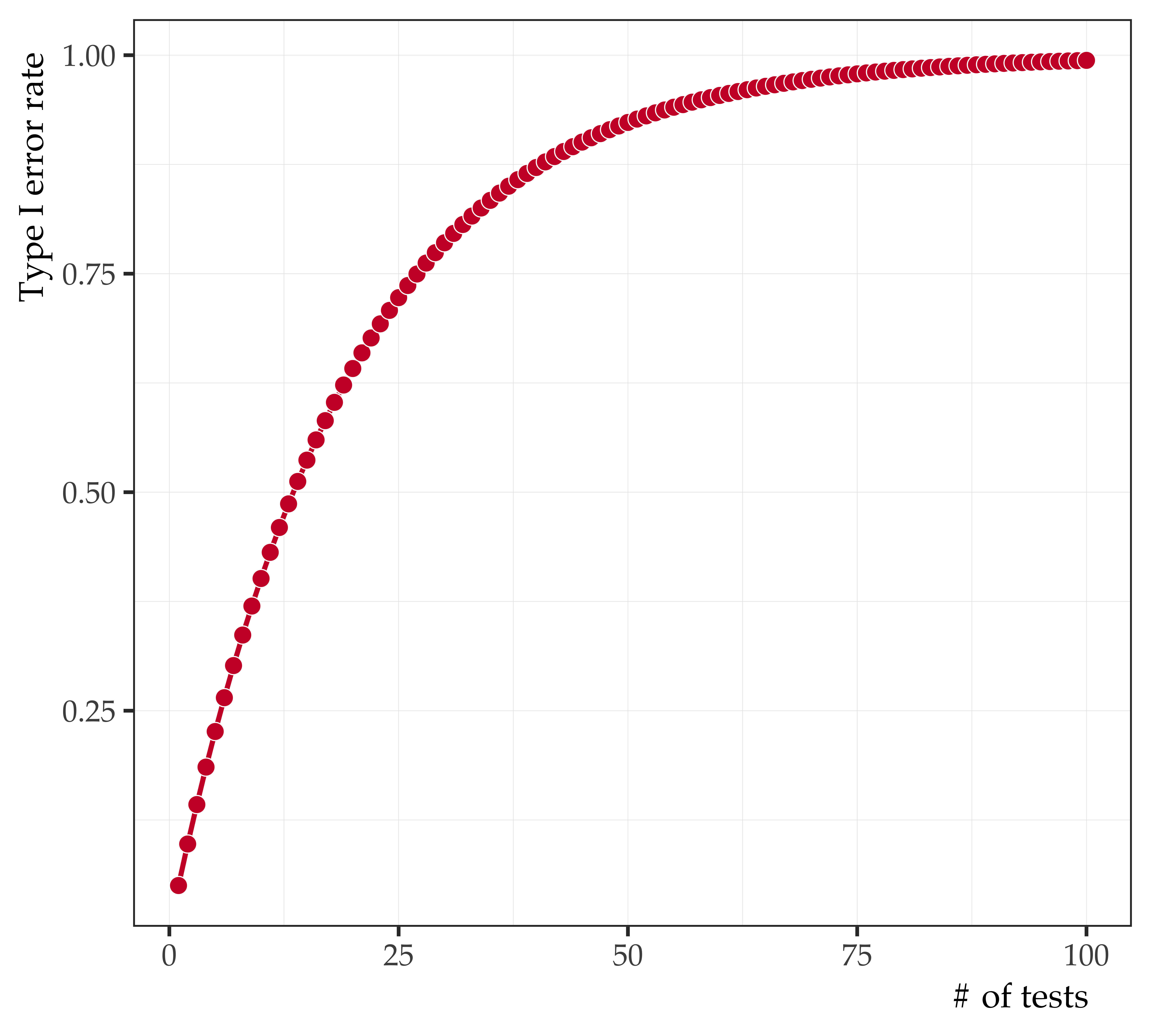
Alpha slippage
- Alpha is the probability of committing a Type I Error
- Experiment-Wise alpha is a function of the Test-Wise alpha and the total number of significance tests conducted:
\[\color{red}{\alpha _{e}} = 1 - (1 - \color{blue}{\alpha _{T}})^\color{green}{k}\]
| αT = | Test-wise alpha |
| k = | Number of significance tests |
| αE = | Experiment-wise alpha |
Alpha slippage
| 0.05 = | Test-wise alpha |
| 10 = | Number of significance tests |
| .40 = | Experiment-wise alpha |
| 0.05 = | Test-wise alpha |
| 20 = | Number of significance tests |
| .64 = | Experiment-wise alpha |
Alpha slippage
| 0.05 = | Test-wise alpha |
| 100 = | Number of significance tests |
| .99 = | Experiment-wise alpha |
| 0.05 = | Test-wise alpha |
| 500 = | Number of significance tests |
| 1.0 = | Experiment-wise alpha |
Alpha slippage
Taking repeated risks
- Every time you do a significance test (at .05) you take a risk of making a Type I Error every 1 in 20 times
- If you do it once you have a 95% chance of being right
- But if you do it multiple times your chances of eventually making a Type I Error greatly increases
- If you have an issue of a journal with 20 articles in it (each using a .05 alpha), the chance of one of those articles reporting a Type I Error is pretty high
Empirical selection of variables
Empirical selection of variables
We should strive to create theoretically specified models that test a priori alternative hypotheses:
- In these models (in a perfect world), all hypotheses are carefully selected, plausible rival hypotheses
- Higher order variables are included when theoretically motivated
We should be discouraged from testing atheoretical ones:
- If you do all possible comparisons, you weaken your statistical power and you get alpha slippage
- When you try to correct for the alpha slippage (by making a more stringent test-wise alpha) you run the risk of committing more Type II Errors
Empirical selection of variables
- There are other techniques in multiple regression that are completely different in basic objectives i.e., empirical selection or exploratory regression techniques
- There are two reasons why we would use exploratory regression techniques that are not based on theory:
- Reason 1: Some people are interested in prediction and not causation, and predictions don’t require theory
- Reason 2: There may be an honest lack of theory in the area you are investigating
Empirical selection of variables
Reason 1: Some people are interested in prediction and not causation, and predictions don’t require theory
- For example, motorcycle ownership increases car insurance rates:
- Causally, this makes no sense
- But for predictive purposes, it does make sense
- Maybe motorcycle owners are riskier car drivers due to personality factors:
- High testosterone?
- Frontal lobe development?
Empirical selection of variables
Reason 2: There may be an honest lack of theory in the area you are investigating
- It might be an entirely new area of scientific investigation
- It might be the case that existing theory was found inadequate or insufficiently supported by the evidence
- However, some people still use exploratory techniques even when they have a theory that they could be testing
- experimenter degrees of freedom
- p-hacking
- fishing expeditions
- pseudoscience
- This is unnecessary and wrong
Empirical selection of variables
How should we do it?
- First, we must design the study:
- We need to sample a broad set of variables, and think as creatively and diversely as you can about what to include
- We need to go beyond the “usual suspects”
- Second, we need to specify the model:
- How do we figure out which variables to include and which should be excluded without a theory?
- Two elementary methods:
- Backward Elimination
- Forward Selection
Empirical selection of variables
Backward elimination
- Include all your variables into a single simultaneous regression model:
- Get b-weights, R2, etc.
- Take a look at all the b-weights
- Try to eliminate any irrelevant variables:
- You are focusing on variables with the smallest effect sizes and the “least significant” b-weights
- Do this one step at time, because multicollinearity may be involved
- Remember this is not theoretically-based and there are no a priori hypotheses
- Re-fit the model with the weakest variable eliminated
- Compare new model to the original one and see if its better:
- Look at the new R2 and then compare the R2 of the model with that variable included with the model with that variable removed, and see if the new model is statistically acceptable
- If you could eliminate that variable, you now look at this model (not the original model) and see which is the next weakest variable
- Try to eliminate this one, and do the same thing all over again
Empirical selection of variables
Backward elimination
Keep doing this until when everything left is significant
When removing something more results in a statistically significant sR2 F-ratio
Then you have to put that last variable back in, and that’s your final model
You are picking off the weakest variables until you can no longer validly eliminate anything else
Empirical selection of variables
Backward elimination - Problems
In true backward elimination, once you eliminate something you can’t go back on that decision
Due to multicollinearity, one variable that was eliminated in an earlier step might now be significant in a new context, but you have no way to know this
Remember significance is often context dependent
Variable A might have not been significant in step 2, but now that variables B, C, and D have been removed it might be significant
Empirical selection of variables
Forward selection
- Correlate all the predictors with the criterion variable (do bivariate correlations of all the predictors with the criterion):
- Pick the one with the best bivariate correlation
- Run the model with this correlation
- Now, you don’t want to include your next largest bivariate correlation from the original correlations that you found:
- Instead, you partial out variable 1 from all remaining variables
- Then you take the one with the biggest sR2 after variable 1 was removed and run the next regression
- To get variable 3, you partial out variable 1 and 2 and look at the variable with the next biggest sR2, and then you put that one in
Empirical selection of variables
Forward selection
- After each step, you take the difference in your R2 values and test it for significance to see if the newly added variable adds a significant amount of variance to the previous model:
- If you have already added variables 1 and 2, and now you want to add variable 3 you need to compare the model with variables 1 and 2 with the model with variables 1, 2, and 3
- So you subtract the R2 and do the semi-partial F-ratio
- Just like an a priori hierarchical procedure!
- Do this until the most recently added variable no longer adds significance variance (sR2) to the model:
- And then throw that variable back!
- Why not test the remaining ones?
- Because you were testing the ones with the largest sR2, so any remaining variables will have lower sR2 and will therefore not add any more significant variance to the model than your last tested variable
Empirical selection of variables
Forward selection - Problems
Similar to Backward Elimination:
- As you put things in there is no way for you to go back and change variables that you already added
- So there is no way of going back and rethinking what you have already done
- Even though variable 1 may have been good in the original context, but now that other variables have been added, it might not make so much sense anymore
- So you can end up in two completely different places using the same data when you use forward selection and backward elimination
Empirical selection of variables
Stepwise regression
- Stepwise Regression is the most popular procedure for exploratory regression:
- It is a combination of forward selection and backward elimination
- Not the same as hierarchical partitioning of variance!
- Basically, you take one step forward, one step back, one step forward, etc.:
- Start with forward selection, then do backward elimination
- Until both of the procedures fail and you can’t add anything profitably and you can’t lose anything profitably
- By combining the two procedures, you get to add something, but then you follow the addition immediately with a backward elimination to see if you can eliminate something else:
- Which you couldn’t do previously with forward selection
- The backward elimination looks at everything, so you can eliminate anything and anytime as long as you don’t lose a significant amount of variance
- So you can eliminate variable 1 in step 8
Empirical selection of variables
hi
Benefits of using exploratory regression techniques:
- You get to proceed in spite of lack of theoretical guidance
- Produce hypotheses/theory building for future research
Major problems involved:
- No a priori theory involved, so the procedure is totally mindless
- You are testing a very large number of variables and you are running a HUGE risk of committing Type I Errors due to massive capitalization on chance
- In fact, you might end up with nothing but Type I Errors!
Reporting results
Reporting
- The main purpose is to explain what you did in a manner that is understandable and reproducible. You should report:
General description:
- Model fit to the data
- Variables included (criterion, predictors)
- Coding/transformations
- Model assumptions/diagnostics
- How you assessed main effects/interactions
- Decision rules (e.g., alpha)
Results
- Model fit
- Main effects (usually NMC)
- Interactions (usually NMC)
- Interpretations:
- directionality
- effect-size
- uncertainty
\(\beta\)
SE
CI
p-val
Reporting
General description
Llompart & Casillas (2016)
Reporting
Results
Llompart & Casillas (2016)
Reporting
General description
Casillas (2015)
Reporting
Results
Casillas (2015)
Reporting
General description
Casillas et al. (2023)
Reporting
Results
Casillas et al. (2023)
References
Berry, W. D., & Feldman, S. (1985a). Multicollinearity. In W. D. Berry & S. Feldman (Eds.), Multiple regression in practice (pp. 37–50). Newbury Park, CA: Sage.
Berry, W. D., & Feldman, S. (1985b). Specification error. In W. D. Berry & S. Feldman (Eds.), Multiple regression in practice (pp. 18–25). Newbury Park, CA: Sage.
Casillas, J. V. (2015). Production and perception of the/i/-/i/vowel contrast: The case of L2-dominant early learners of english. Phonetica, 72(2-3), 182–205. https://doi.org/10.1159/000431101
Casillas, J. V., Garrido-Pozú, J. J., Parrish, K., Arroyo, L. F., Rodrı́guez, N., Esposito, R., Chang, I., Gómez, K., Constantin-Dureci, G., Shao, J., et al. (2023). Using intonation to disambiguate meaning: The role of empathy and proficiency in L2 perceptual development. Applied Psycholinguistics, 44(5), 913–940. https://doi.org/10.1017/S0142716423000310
Cohen, J., & Cohen, P. (1975). Applied multiple regression/correlation analysis for the behavioral sciences. Lawrence Erlbaum.
Figueredo, A. J. (2013a). Empirical selection of variables. Statistical Methods in Psychological Research.
Figueredo, A. J. (2013b). Multiple regression. Statistical Methods in Psychological Research.
Figueredo, A. J. (2013c). Strong inference. Statistical Methods in Psychological Research.
Lewis-Beck, M. (1980). Multiple regression. In M. Lewis-Beck (Ed.), Applied regression: An introduction (pp. 47–74). Newbury Park, CA: Sage.
Llompart, M., & Casillas, J. V. (2016). Lexically driven selective adaptation by ambiguous auditory stimuli occurs after limited exposure to adaptors. The Journal of the Acoustical Society of America, 139(5), EL172–EL177. https://doi.org/10.1121/1.4951704
Schroeder, L. D., Sjoquist, D. L., & Stephan, P. E. (1986a). Multiple linear regression. In L. D. Schroeder, D. L. Sjoquist, & P. E. Stephan (Eds.), Understanding regression analysis: An introductory guide (pp. 29–35). Newbury Park, CA: Sage.
Schroeder, L. D., Sjoquist, D. L., & Stephan, P. E. (1986b). Problems and issues of linear regression. In L. D. Schroeder, D. L. Sjoquist, & P. E. Stephan (Eds.), Understanding regression analysis: An introductory guide (pp. 65–80). Newbury Park, CA: Sage.
Wickham, H., & Grolemund, G. (2016). R for data science: Import, tidy, transform, visualize, and model data. O’Reilly Media.
Bonus - Statistical control in MRC
Some data
'data.frame':   10000 obs. of  5 variables:
 $ age     : num  5 5 5 5 5 5 5 5 5 5 ...
 $ height  : num  36.8 40.9 41.9 40.9 40 ...
 $ score   : num  57.4 55.7 53.9 56.8 53.8 ...
 $ age_c   : num  -6.5 -6.5 -6.5 -6.5 -6.5 -6.5 -6.5 -6.5 -6.5 -6.5 ...
 $ height_c: num  -12.64 -8.56 -7.51 -8.5 -9.42 ...
age height score age_c height_c
1 7.9 40.43 58.87 -3.6 -8.98
2 18.0 56.09 70.63 6.5 6.68
3 5.1 42.76 57.14 -6.4 -6.65
4 17.0 57.87 72.29 5.5 8.45
5 16.8 54.27 68.92 5.3 4.86
6 18.0 54.04 70.00 6.5 4.62
7 11.5 43.96 66.89 0.0 -5.45
8 17.3 58.31 72.03 5.8 8.89
9 16.9 57.62 70.04 5.4 8.21
10 8.8 44.40 60.44 -2.7 -5.01
Call:
lm(formula = height ~ age_c, data = mrc_ex_data)

Residuals:
    Min      1Q  Median      3Q     Max
-11.255  -2.033   0.031   2.013  11.665

Coefficients:
             Estimate Std. Error t value Pr(>|t|)
(Intercept) 49.415790   0.029986  1648.0   <2e-16 ***
age_c        1.261273   0.007989   157.9   <2e-16 ***
---
Signif. codes:  0 '***' 0.001 '**' 0.01 '*' 0.05 '.' 0.1 ' ' 1

Residual standard error: 2.999 on 9998 degrees of freedom
Multiple R-squared:  0.7137,    Adjusted R-squared:  0.7137
F-statistic: 2.493e+04 on 1 and 9998 DF,  p-value: < 2.2e-16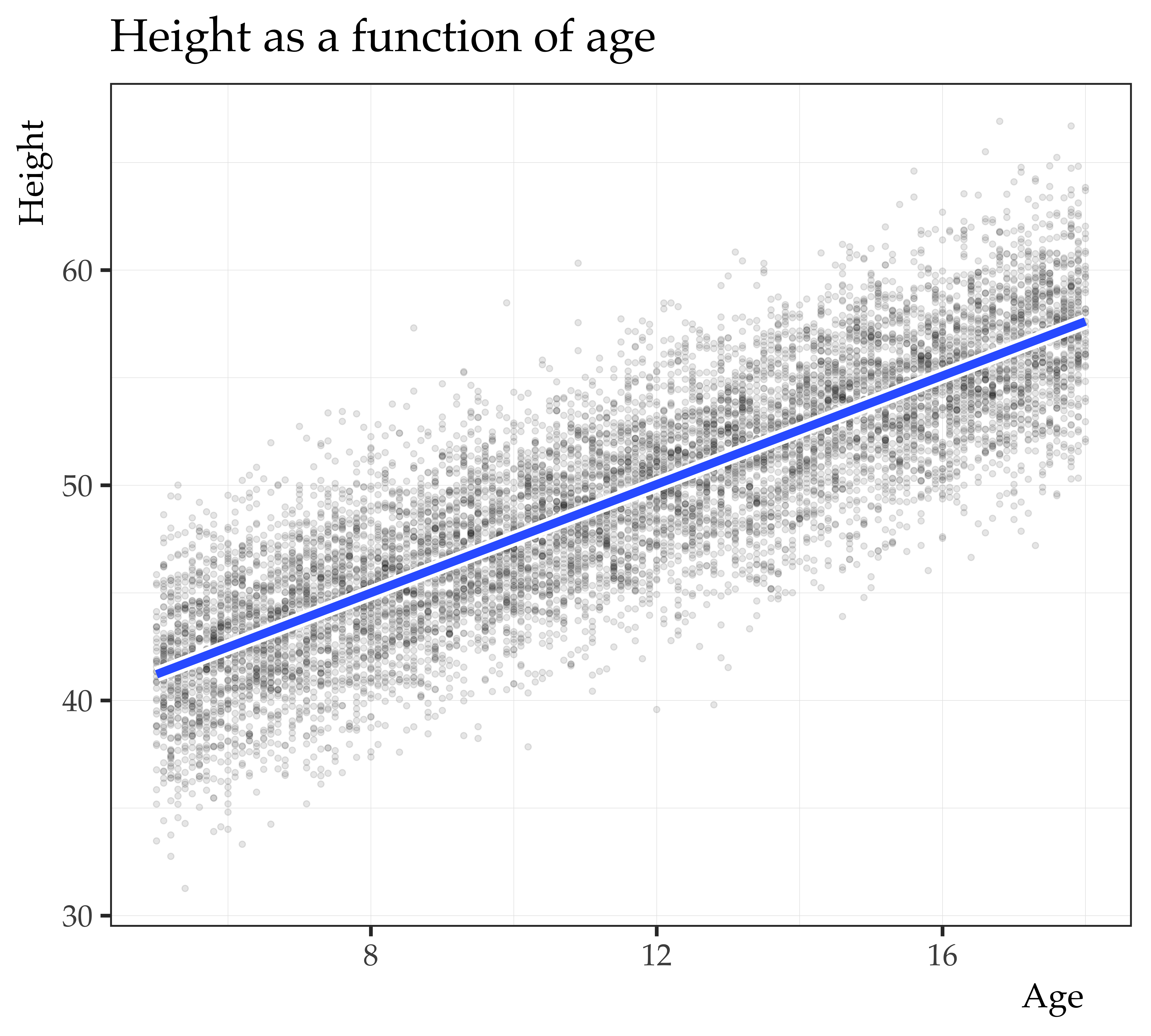
Call:
lm(formula = score ~ age_c, data = mrc_ex_data)

Residuals:
    Min      1Q  Median      3Q     Max
-7.6328 -1.3835  0.0204  1.3758  7.1214

Coefficients:
             Estimate Std. Error t value Pr(>|t|)
(Intercept) 64.367451   0.019954  3225.8   <2e-16 ***
age_c        1.240785   0.005316   233.4   <2e-16 ***
---
Signif. codes:  0 '***' 0.001 '**' 0.01 '*' 0.05 '.' 0.1 ' ' 1

Residual standard error: 1.995 on 9998 degrees of freedom
Multiple R-squared:  0.8449,    Adjusted R-squared:  0.8449
F-statistic: 5.447e+04 on 1 and 9998 DF,  p-value: < 2.2e-16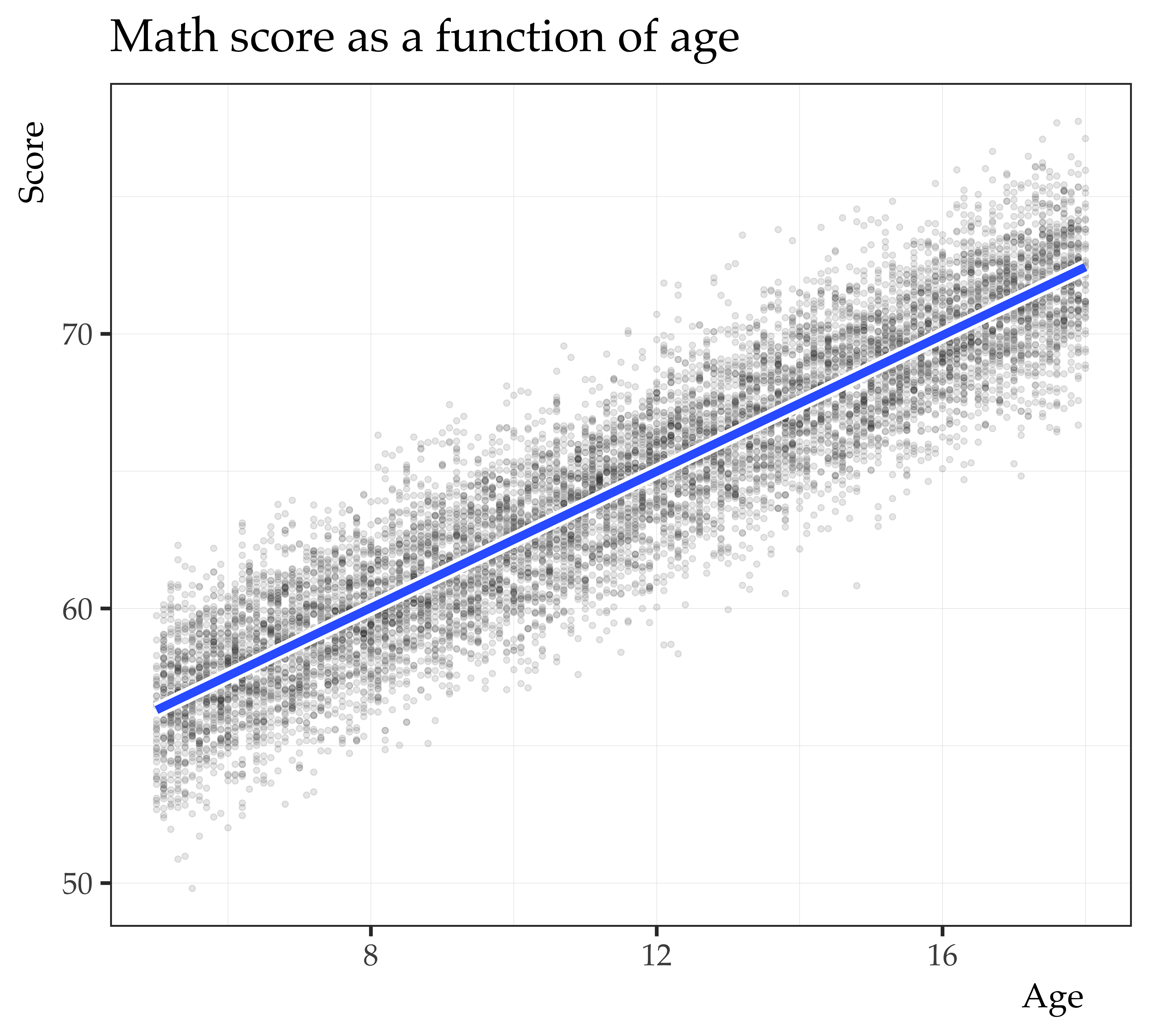
Call:
lm(formula = score ~ height_c, data = mrc_ex_data)

Residuals:
     Min       1Q   Median       3Q      Max
-11.5541  -2.1973  -0.0409   2.1267  12.3640

Coefficients:
             Estimate Std. Error t value Pr(>|t|)
(Intercept) 64.367451   0.031959    2014   <2e-16 ***
height_c     0.701625   0.005703     123   <2e-16 ***
---
Signif. codes:  0 '***' 0.001 '**' 0.01 '*' 0.05 '.' 0.1 ' ' 1

Residual standard error: 3.196 on 9998 degrees of freedom
Multiple R-squared:  0.6022,    Adjusted R-squared:  0.6021
F-statistic: 1.513e+04 on 1 and 9998 DF,  p-value: < 2.2e-16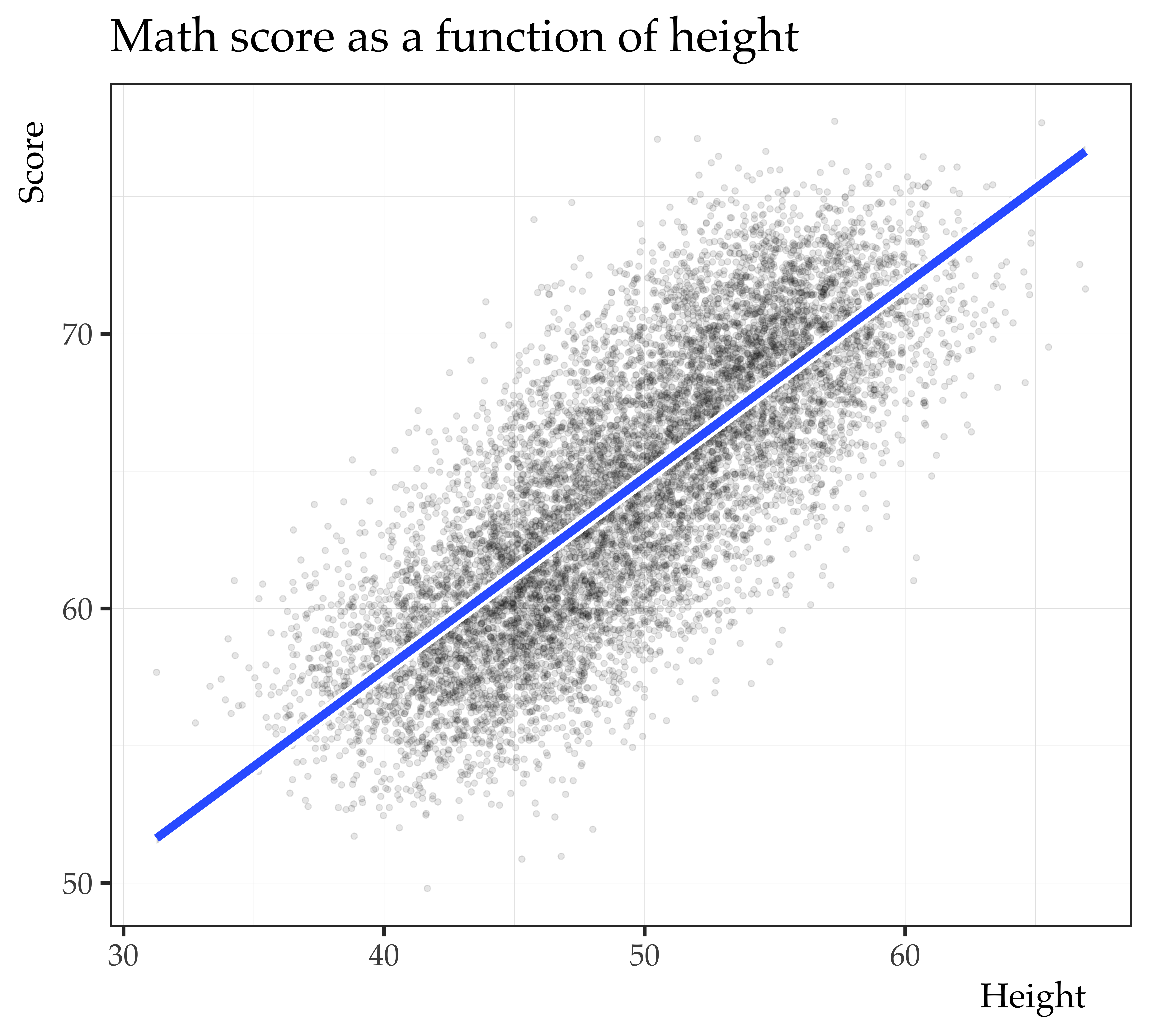
What can we do about this?
Call:
lm(formula = score ~ height_c + age_c, data = mrc_ex_data)

Residuals:
    Min      1Q  Median      3Q     Max
-7.6294 -1.3824  0.0191  1.3743  7.1263

Coefficients:
             Estimate Std. Error t value Pr(>|t|)
(Intercept) 64.367451   0.019955 3225.66   <2e-16 ***
height_c    -0.001730   0.006655   -0.26    0.795
age_c        1.242967   0.009936  125.09   <2e-16 ***
---
Signif. codes:  0 '***' 0.001 '**' 0.01 '*' 0.05 '.' 0.1 ' ' 1

Residual standard error: 1.995 on 9997 degrees of freedom
Multiple R-squared:  0.8449,    Adjusted R-squared:  0.8449
F-statistic: 2.723e+04 on 2 and 9997 DF,  p-value: < 2.2e-16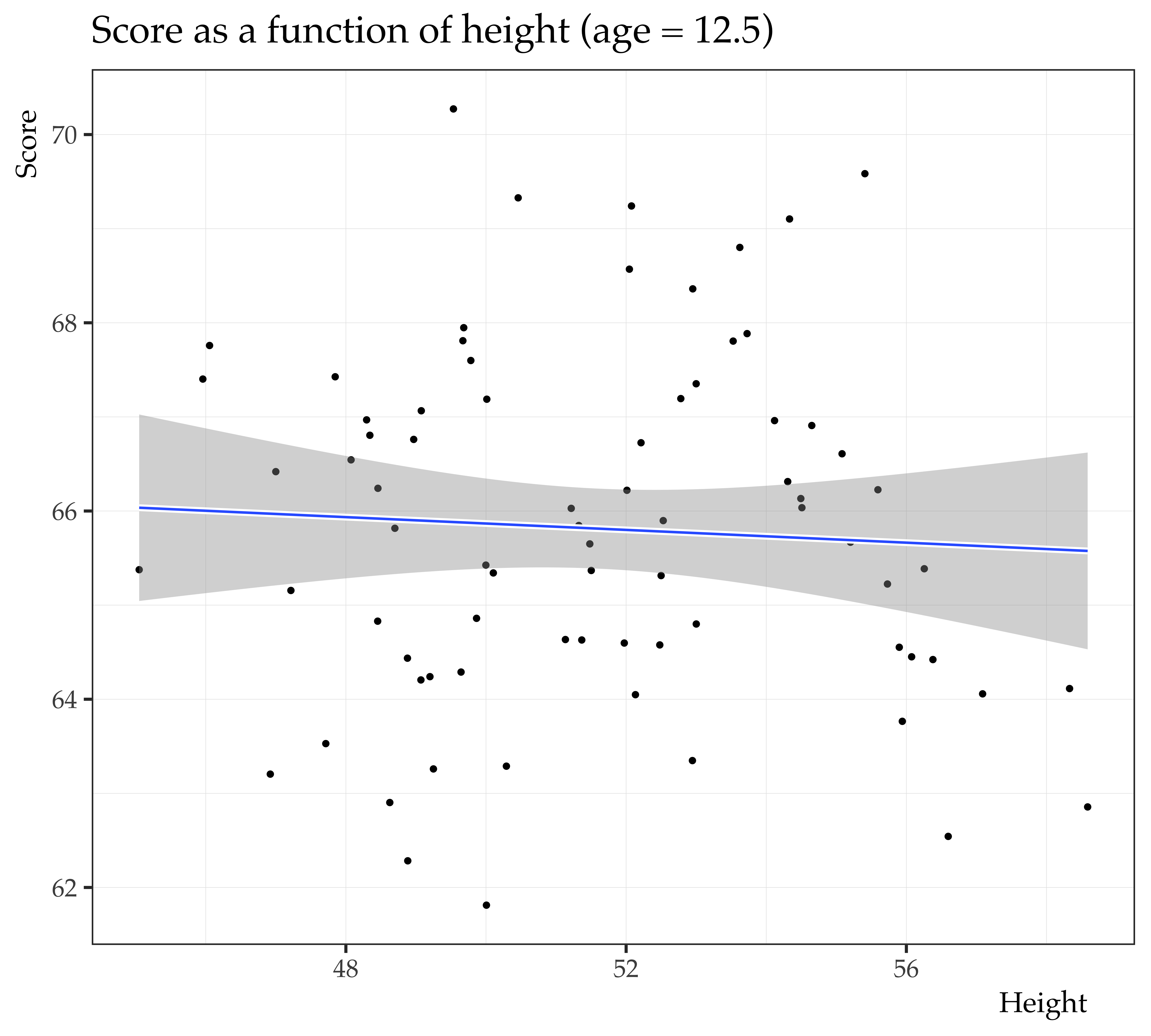
We partial out the spurious relationship between math score
and height by conditioning on age.
